Abstract
Communication of molecular species through dynamic association and/or dissociation at various cellular sites governs biological functions. Understanding these physiological processes require delineation of molecular events occurring at the level of individual complexes in a living cell. Among the few non-invasive approaches with nanometer resolution are methods based on Förster Resonance Energy Transfer (FRET). FRET is effective at a distance of 1-10 nm which is equivalent to the size of macromolecules, thus providing an unprecedented level of detail on molecular interactions. The emergence of fluorescent proteins and SNAP- and CLIP- tag proteins provided FRET with the capability to monitor changes in a molecular complex in real-time making it possible to establish the functional significance of the studied molecules in a native environment. Now, FRET is widely used in biological sciences, including the field of proteomics, signal transduction, diagnostics and drug development to address questions almost unimaginable with biochemical methods and conventional microscopies. However, the underlying physics of FRET often scares biologists. Therefore, in this review, our goal is to introduce FRET to non-physicists in a lucid manner. We will also discuss our contributions to various FRET methodologies based on microscopy and flow cytometry, while describing its application for determining the molecular heterogeneity of the plasma membrane in various cell types.
🔬 Techniques
🔭 Microscopes
✨ Fluorophores
🧪 Sample Preparation
🧪 Reagent Suppliers
🏛️ Research Organizations (ROR)
Affiliated research institutions:
📋 Methods
6.
Methods for Measuring FRET
Fluorescence has many spectroscopic dimensions that can be sensitively monitored and fortunately, the manifestation of FRET is the alteration of these spectroscopic features. Therefore, a multitude of techniques can be employed to measure FRET. Several excellent reviews have been published earlier [ 11 , 13 , 58 , 68 , 69 , 70 , 71 ] where extensive theoretical details are underlined for quantitative analysis of FRET. Types of FRET and the effect of FRET on the spectroscopic features of fluorophores are schematized in Figure 3 . The most notable FRET measurements are based on the following three approaches: (1) Fluorescence intensity based approach; (2) fluorescence lifetime based approach; and (3) fluorescence anisotropy based approach. We have played a seminal role in the development of a ratiometric flow-cytometric FRET (FCET); therefore, FCET will be discussed extensively here, whereas, other FRET methods will be presented through a few mathematical expressions for easy understanding. Figure 3 ( a ) Schematic representation of types of FRET measurements based on photophysical features; and ( b ) This figure illustrates the effect of heteroFRET and homoFRET on fluorescence intensity ( left panels), fluorescence lifetime ( middle panels) and fluorescence anisotropy ( right panels). Here, “D” and “DA” quoted symbols, including the ones in the subscript, represent donor only and FRET samples. In heteroFRET, donors and acceptors are fluorophores with different spectroscopic features. In the upper graph in the left panel, the emission of donor and FRET samples on excitation by the donor excitation wavelength are depicted for simplicity. The green and red curves correspond to the donor and acceptor emission spectra, respectively, in the left panels. In the lower graph in the left panel, there is only a green curve since both the donor and the acceptor are spectroscopically identical. In the middle and right panels, only the time-dependent donor emission (middle) and anisotropy (right) are shown in the absence and presence of the acceptor. The only manifestation of homoFRET is the decrease in anisotropy and no change in fluorescence intensity or fluorescence lifetime of the donor fluorophore. 6.1. Fluorescence Intensity Based Approach 6.1.1.
Show full methods section
6.
Methods for Measuring FRET
Fluorescence has many spectroscopic dimensions that can be sensitively monitored and fortunately, the manifestation of FRET is the alteration of these spectroscopic features. Therefore, a multitude of techniques can be employed to measure FRET. Several excellent reviews have been published earlier [ 11 , 13 , 58 , 68 , 69 , 70 , 71 ] where extensive theoretical details are underlined for quantitative analysis of FRET. Types of FRET and the effect of FRET on the spectroscopic features of fluorophores are schematized in Figure 3 . The most notable FRET measurements are based on the following three approaches: (1) Fluorescence intensity based approach; (2) fluorescence lifetime based approach; and (3) fluorescence anisotropy based approach. We have played a seminal role in the development of a ratiometric flow-cytometric FRET (FCET); therefore, FCET will be discussed extensively here, whereas, other FRET methods will be presented through a few mathematical expressions for easy understanding. Figure 3 ( a ) Schematic representation of types of FRET measurements based on photophysical features; and ( b ) This figure illustrates the effect of heteroFRET and homoFRET on fluorescence intensity ( left panels), fluorescence lifetime ( middle panels) and fluorescence anisotropy ( right panels). Here, “D” and “DA” quoted symbols, including the ones in the subscript, represent donor only and FRET samples. In heteroFRET, donors and acceptors are fluorophores with different spectroscopic features. In the upper graph in the left panel, the emission of donor and FRET samples on excitation by the donor excitation wavelength are depicted for simplicity. The green and red curves correspond to the donor and acceptor emission spectra, respectively, in the left panels. In the lower graph in the left panel, there is only a green curve since both the donor and the acceptor are spectroscopically identical. In the middle and right panels, only the time-dependent donor emission (middle) and anisotropy (right) are shown in the absence and presence of the acceptor. The only manifestation of homoFRET is the decrease in anisotropy and no change in fluorescence intensity or fluorescence lifetime of the donor fluorophore. 6.1. Fluorescence Intensity Based Approach 6.1.1.
Donor Quenching Method
This is the most straight-forward and the easiest method for quick measurement of FRET. It requires an inspection of donor fluorescence in singly (donor only) and doubly (donor-acceptor) labeled samples. The consequence of FRET is the decrease in the fluorescence intensity of the donor in the doubly labeled sample in comparison with the intensity of the donor from the donor only sample. However, this method is error-prone because any quenching observed in the donor fluorescence intensity is assumed to be due to the presence of acceptors. Since the donor intensity is measured in two different samples (donor-labeled and donor-acceptor double-labeled), any difference in the expression level of the labeled antigens, alterations in antibody affinity and spectral cross-talk between the acceptor and donor fluorescence can lead to a difference between the donor intensity in the two samples. Obtaining the mean fluorescence intensity from a large population of cells minimizes the variation in fluorescence at the individual cell level. However, this also prevents donor quenching FRET from providing FRET information on a cell-by-cell basis, thus only mean FRET efficiency representative of a population of cells can be obtained. Therefore, this approach is mainly suitable for flow cytometry or spectrofluorometry based FRET studies [ 10 , 15 , 19 ]. Controls especially to identify competition in antibodies used for labeling the proteins should also be considered. One should make sure that the antibodies do not influence the binding of each other. If any, correction should also be performed for acceptor spill-over in the donor channel [ 15 , 19 ]. Intensities are measured by exciting the sample at the absorption peak of the donor and detecting fluorescence at the emission peak of the donor. Assuming “ F D ” is the fluorescence intensity of the donor sample and “ F DA ” is the fluorescence intensity of the donor and acceptor labeled sample, energy transfer is calculated with the following equation: (5) E = 1 − F DA F D Both F D and F DA have to be background-corrected, i.e ., the fluorescence of unlabeled cells has to be subtracted. 6.1.2.
Acceptor Photobleaching Method
This is mainly a microscopy-based method. Importantly, FRET is estimated from information obtained after imaging a single sample. The general principle is to compare the fluorescence intensity of the donor before and after photodestruction of acceptor species. In the case of occurrence of FRET, there is an increase in the fluorescence intensity of the donor (donor dequenching) after bleaching of acceptors. Since high-intensity laser is used for bleaching of acceptors and acceptor molecule is irreversibly switched off, but remains physically connected to the donor even after bleaching, this approach has a few drawbacks. For example, generation of dark acceptors (non-fluorescent acceptor products, but capable of donor quenching), incomplete photobleaching of acceptor molecules and bleaching of donor species are still possible. Likewise, photobleaching of acceptors can also yield acceptor degradation products with an emission profile similar to that of donor molecules. Importantly, photodestruction of fluorophores means repeated measurements of the same sample is not possible precluding real time information on macromolecules [ 59 , 71 ] although identification of photoswitchable dyes [ 72 ] and fluorescent protein [ 73 ] has offered possibilities for dynamic measurements. Photosensitive acceptors and photostable donors are perfect for the acceptor photobleaching technique. Importantly, precaution should be taken to avoid movement of cells during photobleaching. The mathematical expression for the calculation of energy transfer (E) is analogous to Equation (5) except that F DA is replaced with the fluorescence of donor before acceptor bleaching and F D is substituted by the fluorescence of the donor after photobleaching. 6.1.3.
Sensitized Acceptor Excitation Method
FRET measurement based on quantification of sensitized emission of the acceptor is the most reliable among all intensity-based methods. Sensitized emission of acceptor is the amount of acceptor emission in the FRET channel due to resonance transfer of excitation energy from donor to acceptor [ 59 ]. Simultaneous measurement of individual fluorescence emissions from donor and acceptor from the same sample, in comparison with multi-samples, excludes problems related to variation, such as changes in donor density or fluorescence quantum yield [ 59 , 68 ]. Nonetheless, FRET estimations are more accurate and easier to perform in a case when donor and acceptor emissions are well separated. Otherwise, this method invites the introduction of several correction factors related to fluorophore cross-talk, i.e ., the reciprocal excitation of donor and acceptors at the excitation wavelength of the other dye, and bleed-through of fluorescence emission of the donor and the acceptor to detection channel corresponding to the other dye. Independent control samples of donor and acceptor can help compensate the issues related to the above problems. Numerous methods have evolved with a goal of quantifying sensitized acceptor signal. Although quantitative approaches determining the FRET efficiency rigorously are preferred [ 53 ], semi-quantitative method providing uncalibrated FRET indices with dubious theoretical background also abound in the literature [ 59 ]. FRET indices are instrument dependent relative values designed according to the aims of studies. They are qualitative in nature, however, some of them seem to be more sensitive and consistent in cases where FRET efficiency based methods tend to suffer, for instance, when the ratio of donor to acceptor is lower than 1 [ 59 ]. With its simple mathematical framework, these approaches would seem rather attractive to biologists who are more concerned about learning the possibility of interactions between two macromolecules in a simple “yes” or “no” format or knowing the consequence of a biological response in the association of proteins in relative terms. Based on the literature, methods for measurement of sensitized emission can be categorized into three groups with the basic difference being the process of analyzing FRET signals: (1) Two-channel emission or excitation ratio measurement; (2) three-channel emission measurement; and (3) spectral analysis for FRET.
Two-Channel Emission or Excitation Ratio Measurement
Two channel emission ratio measurement has been applied a lot both in microscopy [ 74 , 75 ] and flow cytometry [ 76 , 77 ] as sensors of protein–protein interactions. Basically, the practice is to illuminate the doubly (donor and acceptor) labeled sample with the donor excitation wavelength, then, collect the signals in both donor and FRET channels, i.e ., in the wavelength range corresponding to the emission peak of the donor and acceptor, respectively. A FRET index defined as the ratio of fluorescence intensities in the FRET and donor channels are widely used owing to the fact that the ratio is fairly consistent [ 19 , 52 , 78 ]. An alternative two-channel excitation ratio measurement has also been described before, where measurements at the emission wavelength of acceptor were taken upon consecutive excitation of the FRET sample with donor (FRET channel) and acceptor (acceptor channel) wavelengths. In this case, a parameter proportional to the FRET efficiency is expressed as the ratio of fluorescence in the FRET channel to the fluorescence in the acceptor channel [ 78 , 79 ]. Primarily, the above methods are ignorant to multiple cross-talks and bleed-through features of fluorophores such as direct excitation of the acceptor at the donor absorption wavelength. However, these methods are very useful as long as the ratio of the concentrations of donors and acceptors is constant such as in intramolecular FRET studies [ 52 , 54 ] involving FRET-sensors.
Three-Channel Emission Measurement
Three-channel emission measurement requires collection of three independent signals from the same sample. These signals differ either in the wavelength of excitation or in a spectral range of detectors for recordings. In fact, this method is similar to the two-channel measurement with an additional third channel making rigorous deductions of non-FRET signals possible. Numerous studies have been published representing such a set-up with varying level of stringency with regards to cross-talk or bleed-through corrections [ 59 ]. For three-channel measurement, assessment of FRET has been demonstrated both in terms of FRET indices [ 52 , 53 , 80 , 81 ] and FRET efficiencies [ 15 , 54 , 68 , 69 , 82 , 83 ]. Measurements require collection of signals for donor alone, acceptor alone and doubly (donor-and-acceptor) labeled samples under the same circumstances. Below, we will describe three of the most popular FRET index based three-channel measurements with FRET terminologies used by the respective authors: (a) Corrected FRET ( F c ) method: This method was introduced by Youvan et al ., for epifluorescence microscope [ 80 ]. They simply generated a FRET image corrected for fluorescence from background and bleed-through. However, the contribution of reciprocal cross-talk excitation in donor and acceptor channels, which were minimal in their case, was not considered during the calculation. Similarly, the method does not perform normalization for concentration of donors and acceptors. Therefore, it inherently suffers from the issues related to variability in fluorophore concentration. In fact, even at the same FRET efficiency, the FRET signal is different for samples in which various concentrations of donors and acceptors are used. Thus, it is suitable under conditions when the donor to acceptor concentration is constant or known beforehand. The corrected FRET was expressed in the following form: (6) F c = F f – [ ( F d / D d ) × D f ] – [ ( F a / A a ) × A f ] In Equation (6), F , D and A represent FRET, Donor and Acceptor channels, respectively, whereas subscripts “f”, “d” and “a” represent FRET, donor and acceptor samples, respectively. The spectral bleed-through for donor ( F d / D d ) and acceptor ( F a / A a ) are calculated from donor only and acceptor only samples, respectively. It is also assumed that the images were background subtracted in the above equation. (b) FRET net (FRETN) method: Gordon et al . presented a FRETN method to overcome the underlying problem with the F c method. F c is linearly proportional to the concentration of fluorophores; therefore, they proposed that Equation (6) should be additionally normalized by the product of donor and acceptor signals [ 54 ]. This new method, however, overcompensates by dividing the F c value with both donor and acceptor intensities. Therefore, FRET values flatten out at higher donor and acceptor intensities whereas it is fairly sensitive at low donor and acceptor intensities. Thus, this method generates FRET values with high standard error (80%) affected by concentrations of donors and acceptors [ 84 ]. (7) FRETN = F c / G × D f × A f The notations in Equation (7) are similar to that of Equation (6). A constant “ G ” is a parameter which relates the loss of donor signal to the increase in acceptor signal as a result of FRET (please refer to Equations (15) and (16) for “ G ” which is equivalent to “α” in the section below). (c) Normalized FRET (N FRET ) method: In order to reduce the inconsistency of the FRETN method, Xia et al introduced the normalization procedure for F c with the product of the square root of donor and acceptor signals [ 84 ]. This renders FRET independent of local concentration of fluorophore. However, N FRET is still not linear with changes in E values and fractional occupancy; therefore, it is not adequate for stoichiometric measurements of binding interactions [ 85 ]. (8) N FRET = F c / D f × A f Several other methods have also been published where the basis of normalization of FRET value is with acceptor concentration [ 81 , 86 ]. Experimental results obtained using FRET indices from different instruments are not comparable because FRET indices depend on system parameters such as excitation intensities and detection efficiencies of the instrument [ 21 ]. Therefore, it is more relevant to express FRET through an instrument-independent, but quantitative parameter such as FRET efficiency. Assuming that the FRET-pair is red-shifted, which minimizes autofluorescence [ 27 ], and the contribution of background is negligible, FRET efficiency can be easily computed by solving a set of three linear equations corresponding to the signals from a FRET sample. They are expressed as a function of unquenched donor ( I D ), the FRET efficiency ( E ) and intensity from the acceptor in the absence of FRET (I A ). To maintain consistency, we are using similar terminologies as in our previous papers [ 15 , 68 , 69 , 82 ]. The following equations are based on FCET [ 15 , 68 ], although, we also implemented it in microscopy [ 69 , 70 ]. First, we would like to introduce the correction factors, which need singly labeled samples of donor and acceptor, so that it becomes easy to follow the equations. Correction factors result from spill-over and cross-excitation between donor and acceptor fluorophores, thus, are necessary for eliminating non-FRET signals. In a general case, four different “ S ” factors are used, namely S 1 , S 2 , S 3 and S 4 . S 1 and S 3 characterize the spill-over of donor intensity to the FRET ( I 2 ) and acceptor ( I 3 ) channels, respectively, and are determined using donor only labeled sample. (9) S 1 = I 2 I 1 , S 3 = I 3 I 1 S 2 and S 4 characterize the spill-over of acceptor intensity to the FRET ( I 2 ) and donor ( I 1 ) channels, respectively, and are determined using acceptor only labeled sample. (10) S 2 = I 2 I 3 , S 4 = I 1 I 3 where I 1 , I 2 and I 3 correspond to intensities measured in the donor, FRET and acceptor channels, respectively. The excitation (λ ex ) and emission (λ em ) wavelength for each of the intensities is defined in the parenthesis of Equations (11)–(13). For instance, the abbreviation in the symbol (λ ex,D ; λ em,D ) means excitation at the wavelength corresponding to the donor absorption band, and emission detected at the wavelength corresponding to the donor emission wavelength range. The uppercase letters “D” or “A” in the symbols represent donor and acceptor, respectively. (11) I 1 ( λ ex , D ; λ em , D ) = I D ( 1 − E ) + I A × S 4 + I D × E × α × S 4 S 2 (12) I 2 ( λ ex , D ; λ em , A ) = I D ( 1 − E ) × S 1 + I A × S 2 + I D × E × α (13) I 3 ( λ ex , A ; λ em , A ) = I D ( 1 − E ) × S 3 + I A + I D × E × α × 1 S 2 × ϵ λ A D ϵ λ D A ϵ λ D D ϵ λ A A Here, “ϵ” stands for molar absorption coefficient of “D” and “A” molecules shown by the upper indices at donor ( λ ex , D ) or acceptor wavelengths ( λ ex , A ). Often, S 3 , S 4 and the molar absorption ratio, ( ϵ λ A D ϵ λ D A ϵ λ D D ϵ λ A A ) , are negligible, as with the Cy3-Cy5 FRET-pair when measured on a FACSCalibur (BD Bioscience, San Jose, CA, USA). Thus, solving Equations (11)–(13) would yield “E” in the following form (see references [ 15 , 68 ] for the derivation): (14) E = I 2 − I 1 S 1 − I 3 S 2 α I 1 + I 2 − I 1 S 1 − I 3 S 2 It is also clear from the above set of equations that calculating “E” in ratiometric FRET requires determining a factor “α”, which has been widely used as “G” in microscopy, to correct for the differences in the quantum yield of the donor and acceptor and in the detection efficiencies of the donor in the donor channel and the acceptor in the FRET channel. “α” relates the loss of donor fluorescence to the sensitized emission of the acceptor. Classically, “α” is expressed as in the equation below: (15) α = Q A η A Q D η D where “ Q D ” and “ Q A ” are the fluorescence quantum yields of the donor and acceptor fluorophores, respectively, and “η D ” and “η A ” are the detection efficiencies of the donor in the donor channel and the acceptor in the FRET channel, respectively. Since both the quantum yield and the detection efficiencies are difficult to determine or calculate, numerous ways of calculating “α” factor have been reported previously though not without the challenges owing to the underlying variables. The interested readers are referred to the cited references for learning various approaches of determining “α” factor in microscopy [ 21 , 55 , 69 , 70 , 83 , 85 ] and flow cytometry [ 15 , 55 , 65 , 87 ]. One of the simplest approaches for calculating “α” is based on labeling two separate samples. One of the samples is labeled with a donor-tagged antibody and the other with an acceptor-tagged antibody. In such a case, “α” can be calculated according to the following equation: (16) α = I 2 , A I 1 , D × B D B A × L D L A × ϵ λ D D ϵ λ D A where I 2,A and I 1,D are the intensity of the acceptor-labeled sample measured in the FRET channel and the intensity of the donor-labeled sample measured in the donor channel, respectively. Likewise, “ B D ” and “ B A ” are the mean number of epitopes labeled by the donor-conjugated and acceptor-conjugated antibodies, respectively, and “ L D ” and “ L A ” denote the labeling ratios ( i.e ., number of fluorophores/antibody) of the donor-conjugated and acceptor-conjugated antibodies, respectively. For the sake of simplicity, it is advisable to label the same epitope with the donor- and acceptor-conjugated antibodies, so that B D = B A . Unfortunately, the method described above requires measuring a large number of cells, so that the mean intensities ( I 2,A and I 1,D ) are reliably determined, which is difficult to achieve in microscopy. Alternatively, “α” can be calculated by labeling the same membrane protein with two non-competing antibodies binding to distinct epitopes but far enough to avoid any occurrence of FRET. One of the antibodies should be donor-tagged, while the other should be acceptor-conjugated. This approach ensures that the B D / B A ratio is equal to 1 since the intensities I 2,A and I 1,D are measured on the same cells. Thus, “α” can be easily calculated from Equation (16) with B D / B A = 1. If the requirement for no FRET cannot be met, the energy transfer taking place between the donor- and acceptor-labeled antibodies has to be taken into consideration [ 55 , 88 ]. Despite the use of such a systematic method for calculating “E”, satisfactory results are still difficult to obtain for proteins with low expression levels. Thus, in cases when the signal to noise ratio is very low, accurate FRET calculations require cell-by-cell correction for autofluorescence and selection of a FRET-pair with long emission wavelength. This improvement reduces the dispersion of FRET histograms and thereby improves the sensitivity of FRET analysis [ 15 , 27 , 69 ]. Likewise, we have also recently introduced an efficient method applicable in such cases called Maximum Likelihood Estimation (MLE) of FRET efficiency. The method is based on the assumption that photon detection by detectors follows Poissonian statistics [ 63 ]. We developed a computational tool applying the Poisson function to I 2 intensity expressed as a function of I 1 and I 3 after solving Equations (11)–(13). The method thus predicts the joint probability of photon numbers received by the donor, FRET and acceptor channels. The presented algorithm assigns a single FRET efficiency based on the likelihood of all three measured intensities to each pixel. Therefore, outlier pixels with low probabilities for the determined FRET efficiency can be easily excluded from the analysis thus improving the accuracy of the calculation significantly. The only drawback is that MLE of FRET requires a dataset of at least 100 pixels, corresponding to region of 1 μm × 1 μm assuming a pixel size of 100 nm, for accurate determination of FRET efficiency; therefore, pixel-by-pixel documentation of “E” in an image is not possible. However, heterogeneity in spatial subsets due to biological variance can be explored when regions of interest are selected for analysis in the cell. With physiological settings, known to have low photon numbers due to weak expression of proteins and with abundant outer pixels of both biological and instrumental origins, we noted that MLE of FRET efficiency exceeds the performance of both pixel-by-pixel and total intensity based FRET approaches. The traditional method of calculating “E” suffers from distortion generated by detector noise, thus uncertainties prevail while calculating “E” for weakly expressed proteins. In fact, the FRET histogram would be wide and asymmetrical with large variance making “E” meaningless. Readers interested in the theoretical and mathematical background on this method can review our recently published paper [ 63 ]. The method was developed for confocal microscope; however, we do not see any reason why it cannot be adapted to flow cytometry as long as photon counting detectors are used.
Spectral Analysis for FRET
The idea of spectral analysis for FRET was borrowed from remote sensing and satellite imaging techniques [ 89 ]. The approach is to record a set of images in a series of wavelength bands, also referred to as lambda (λ) stacks. It is assumed that each fluorophore has its own specific spectral signature, which can be identified within the λ stack. With these signature reference spectra of the fluorophores and autofluorescence, the contribution of each fluorophore and autofluorescence in a mixed spectrum, as in a FRET sample, can be easily identified, even with a high degree of spectral and spatial overlap, using linear unmixing algorithms [ 90 , 91 , 92 , 93 , 94 , 95 ]. Taking advantage of this feature, several FRET approaches have been described; in fact, in many of the cases spectral imaging was just used as an addendum to the traditional FRET approaches to increase accuracy [ 90 , 92 , 93 ]. However, separating acceptor bleed-through from FRET signal is very difficult to obtain with linear unmixing because of their identical emission spectrum. This approach is primarily suitable for two-photon microscopy where judicious selection of excitation wavelength could be achieved easily thus circumventing acceptor cross-excitation [ 96 ]. Typically, the emission spectra of the donor and acceptor contain all the information regarding the concentration of fluorophores and the FRET efficiency [ 97 ]. Despite the possibility in increased sensitivity offered by spectral FRET measurement, the whole approach is complicated and requires special hardware for recording “λ” stacks. Additionally, the idea to distribute emission spectra in a series of spectral intervals to multiple detector channels also demands modification in instrumental settings (e.g., laser power, line averaging or pixel dwell time) for each of these channels potentially making each of the acquired images noisy [ 94 ]. Spectral FRET analysis is primarily used in microscopy; however, it is also feasible in spectrofluorometry [ 92 , 95 ] and spectral flow cytometry. 6.1.4.
Donor Photobleaching Method
Monitoring the photobleaching kinetics of donor in the presence or absence of acceptor also offers a simple approach to determine FRET. Photobleaching occurs from the excited state of a fluorophore. The stability of donors increases due to decrease in the availability of the excited state donor molecules when nearby acceptors are present due to FRET. Consequently, energy transfer decreases the rate of photobleaching and increases the bleaching time constant of the donor [ 57 , 82 , 98 ]. In contrast to the acceptor photobleaching technique, this approach requires a photolabile donor and photostable acceptor allowing determination of FRET efficiency [ 58 , 68 , 99 ]. This method also offers the advantage of being insensitive to expression density of proteins under investigation (since the kinetics of bleaching are measured which is assumed not to be influenced by the expression levels unless the expression level alters FRET), however, other environmental factors, like oxygenation, fluorophore concentration, temperature, etc., can still influence donor photobleaching. The measurements are not self-controlled; therefore, mixing singly and doubly labeled cells and measuring them on the same slide sequentially or simultaneously for the bleaching kinetics would reduce errors due to the above factors. Since pixel-by-pixel bleaching time can differ due to molecular environment or other factors, it is considered to be more effective with wide-field microscopy instead of confocal laser scanning microscopy [ 68 , 100 ]. Donor photobleaching can be correlated to the FRET efficiency using the equation below: (17) E = 1 − T D T DA In Equation (17), T D and T DA stands for the photobleaching time constant of donor in the absence and presence of acceptor, respectively. For calculating time constants, a sequence of images of donor from the corresponding samples are taken with donor-specific optical filter sets while bleaching the donor until it reaches the level of background. Since images are recorded at different times, the image stacks store the time-dependent fluorescence of the donor, or bleaching curve, which is fitted by the following exponential function resulting in the desired photobleaching constants [ 49 , 68 , 69 , 82 ]. (18) I t = I 0 e − t T + b g where I t is the time dependent donor fluorescence intensity, I 0 is the donor intensity before bleaching, t is time, T is the bleaching time constant and bg is the background. In some cases, a single exponential function is not sufficient to achieve reasonable fits. In these cases a double exponential fit may be carried out [ 57 ]. 6.2.
Fluorescence Lifetime Based Approach
Fluorescence lifetime (τ) characterizes the time spent by fluorescent species at the excited state before exiting to the ground state by radiative and non - radiative mechanisms. Therefore, it is inversely proportional to the sum of all the kinetic processes: rate constant of fluorescence emission ( k f ), rate constant of FRET ( k FRET ), if present, and rate constant of all other non-fluorescent mechanisms ( k nf ), responsible for relaxation of the excited fluorophore. (19) τ D = 1 k f + k nf , τ DA = 1 k f + k FRET + k nf where τ D and τ DA are the fluorescence lifetime of the donor in the absence and presence of the acceptor ( i.e ., FRET), respectively. A convenient way to measure fluorescent lifetime is to determine fluorescence emission decay which follows first-order kinetics for a simple fluorophore [ 101 ]. Fluorescence lifetime is mathematically defined as the time taken by a population of excited molecules to decay by a factor of e (or to 37% of the initial population) [ 62 , 102 ]. Each fluorophore has its own characteristic fluorescence decay pattern like unique spectral fingerprints. FRET introduces a new de-excitation pathway and consequently accelerates the relaxation process. Therefore, with the increase in the rate of FRET, the donor lifetime decreases because of proximity to acceptors [ 82 ]. Understandably, fluorescence lifetime provides a direct measure to determine FRET. For an excited fluorophore, the rate of return to the ground state depends on their number in the excited state times a rate constant, therefore, “E” can be expressed from fluorescence lifetimes as below: (20) d [ D * ] dt = − [ k f + k nf ] [ D * ] = − 1 τ D [ D * ] (21) d [ D FRET * ] dt = − [ k f + k FRET + k nf ] [ D FRET * ] = − 1 τ DA [ D FRET * ] (22) E = k FRET k FRET + k f + k nf = k FRET + k f + k nf − ( k f + k nf ) k FRET + k f + k nf = 1 − τ DA τ D Equations (20) and (21) correspond to the first-order decay kinetics of donor only and FRET samples. In the above equations, [ D * ] and [ D FRET * ] represent concentration of donors at excited state for donor and FRET samples, respectively, at time “t”. The rate constants ( k f , k nf and k FRET ) are described in Equation (19).
Fluorescence lifetime based FRET
(FL-FRET) can be carried out in a microscope, a spectrofluorometer or a flow cytometer. An important feature of FL-FRET is its ability to predict the fraction of acceptor-bound donor based on the fluorescence decay curve [ 19 , 94 ]. Fluorescence lifetime is also independent of fluorophore concentrations, emission of acceptors and instrumental factors. Therefore, FL-FRET does not suffer from the major issues seen in intensity analysis based FRET methods like spectral spillover, differences in local concentrations of fluorophores, variation in excitation intensity and exposure duration [ 35 , 62 , 101 ]. This means that the whole FRET experiment is simplified, requiring less experimental controls and normalization procedures. Therefore, it is highly valuable under conditions where the above experimental parameters are hard to control or determine. Fluorescence lifetime is determined by energetically unstable state of a fluorophore; therefore, it is sensitive to perturbations related to temperature, polarity, refractive index of medium and various quenching effects [ 35 , 102 ]. The exploitation of FL-FRET in microscopy also makes it possible to map the spatial and temporal lifetime dynamics of the molecule with increased accuracy. However, FL-FRET requires long acquisition times in microscopy. Additionally, most biologically relevant fluorophores exhibit lifetimes of nanoseconds. Therefore, fluorescence lifetime measurements also demand sophisticated and expensive instrumentation [ 103 ]. 6.3.
Fluorescence Anisotropy Based Approach
Fluorophores are randomly oriented in space and time even in the case of fluorescently labeled plasma membrane protein. Imagining that polarized light excites a stationary fluorophore, the consequent fluorescence emission is also polarized in the same plane. Exposure to a polarized light typically leads to excitation of only a fraction of the total population of fluorophores. This is because fluorophores are free to enjoy any random orientations and only those fluorophores are excited whose absorption transition dipole is aligned suitably or nearly parallel to the polarization plane of the excitation source, a process called photoselection. Furthermore, during the excited state, fluorophores can demonstrate reorientation before they lose energy through both radiative and non-radiative mechanisms including FRET. Consequently, the emitted light is depolarized in comparison with the polarized excitation source [ 11 ]. Fluorescence anisotropy (r) defines how much fluorescence emission is polarized after polarized excitation. If a fluorophore is illuminated with a vertically polarized light, then, both vertical ( I v ) and horizontal ( I h ) emissions should be collected. Processes leading to depolarization of emission are then characterized by these two intensities based on anisotropy calculated according to Equation (23). (23) r = I v − I h I v + 2 I h Anisotropy is sensitive to the size and shape of the molecule, rigidity or fluidity of the molecular environment, rotational motion and molecular association events [ 13 ]. Larger fluorophores will have slower mobility whereas smaller sized fluorophores will tumble and rotate faster. Therefore, larger species will have high anisotropy while small species will have low anisotropy values. However, it is not only the rotation of fluorophores that can alter anisotropy. Typically, FRET also alters the anisotropy of the fluorophore ( Figure 3 ) [ 11 , 13 ]. HeteroFRET shortens the donor's lifetime; therefore, the donor has less time to rotate during the excited state lifetime before emitting a photon. Consequently, donor emission is hyperpolarized (relative to the case when no heteroFRET takes place) resulting in an increase of anisotropy. HomoFRET does not affect lifetime but rather leads to the transfer of energy between like molecules. Each homoFRET step depolarizes the excited population since the acceptors excited by homoFRET are not parallel to the donor. Since the donor and the acceptor are spectroscopically identical, i.e. , their fluorescence is indiscriminable, the eventual emission is less polarized with a resultant decrease in anisotropy. Importantly, ensemble fluorescence intensity and lifetime of donor are reduced in heteroFRET but remain unchanged in homoFRET. The extent of depolarization of the fluorophore emission in homoFRET depends on the oligomerization state of the proteins. The larger the number of molecules in a cluster, the lower the anisotropy of the overall fluorescence emission is [ 13 , 14 ]. This feature makes homoFRET a useful tool in the quantitative analysis of large protein clusters [ 14 , 104 ]. However, polarization artifacts induced by sample and instrumental factors easily influence this method. Optical lenses with high numerical aperture (>1) are also found to cause significant depolarization of the emission light. The apparent anisotropy decreases with the increase in numerical aperture of the objective lens. Therefore, objectives with lower numerical aperture are more accurate for anisotropy measurements although with loss in resolution and sensitivity [ 105 ]. Anisotropy measurements require highly expressed proteins because the emission signals from the fluorophores are significantly reduced due to the polarizer and also as a result of splitting of the emission signals into vertical and horizontal components [ 62 , 106 ]. Additionally, anisotropy is not very sensitive to the FRET efficiency. It is only suitable for providing information on the presence or absence of FRET, but cannot be used to measure small changes in FRET [ 62 , 94 ]. Nonetheless, both microscopic and flow-cytometric applications of anisotropy can be found in the literature [ 13 , 104 ].
6.1.1.
Donor Quenching Method
This is the most straight-forward and the easiest method for quick measurement of FRET. It requires an inspection of donor fluorescence in singly (donor only) and doubly (donor-acceptor) labeled samples. The consequence of FRET is the decrease in the fluorescence intensity of the donor in the doubly labeled sample in comparison with the intensity of the donor from the donor only sample. However, this method is error-prone because any quenching observed in the donor fluorescence intensity is assumed to be due to the presence of acceptors. Since the donor intensity is measured in two different samples (donor-labeled and donor-acceptor double-labeled), any difference in the expression level of the labeled antigens, alterations in antibody affinity and spectral cross-talk between the acceptor and donor fluorescence can lead to a difference between the donor intensity in the two samples. Obtaining the mean fluorescence intensity from a large population of cells minimizes the variation in fluorescence at the individual cell level. However, this also prevents donor quenching FRET from providing FRET information on a cell-by-cell basis, thus only mean FRET efficiency representative of a population of cells can be obtained. Therefore, this approach is mainly suitable for flow cytometry or spectrofluorometry based FRET studies [ 10 , 15 , 19 ]. Controls especially to identify competition in antibodies used for labeling the proteins should also be considered. One should make sure that the antibodies do not influence the binding of each other. If any, correction should also be performed for acceptor spill-over in the donor channel [ 15 , 19 ]. Intensities are measured by exciting the sample at the absorption peak of the donor and detecting fluorescence at the emission peak of the donor. Assuming “ F D ” is the fluorescence intensity of the donor sample and “ F DA ” is the fluorescence intensity of the donor and acceptor labeled sample, energy transfer is calculated with the following equation: (5) E = 1 − F DA F D Both F D and F DA have to be background-corrected, i.e ., the fluorescence of unlabeled cells has to be subtracted.
6.1.2.
Acceptor Photobleaching Method
This is mainly a microscopy-based method. Importantly, FRET is estimated from information obtained after imaging a single sample. The general principle is to compare the fluorescence intensity of the donor before and after photodestruction of acceptor species. In the case of occurrence of FRET, there is an increase in the fluorescence intensity of the donor (donor dequenching) after bleaching of acceptors. Since high-intensity laser is used for bleaching of acceptors and acceptor molecule is irreversibly switched off, but remains physically connected to the donor even after bleaching, this approach has a few drawbacks. For example, generation of dark acceptors (non-fluorescent acceptor products, but capable of donor quenching), incomplete photobleaching of acceptor molecules and bleaching of donor species are still possible. Likewise, photobleaching of acceptors can also yield acceptor degradation products with an emission profile similar to that of donor molecules. Importantly, photodestruction of fluorophores means repeated measurements of the same sample is not possible precluding real time information on macromolecules [ 59 , 71 ] although identification of photoswitchable dyes [ 72 ] and fluorescent protein [ 73 ] has offered possibilities for dynamic measurements. Photosensitive acceptors and photostable donors are perfect for the acceptor photobleaching technique. Importantly, precaution should be taken to avoid movement of cells during photobleaching. The mathematical expression for the calculation of energy transfer (E) is analogous to Equation (5) except that F DA is replaced with the fluorescence of donor before acceptor bleaching and F D is substituted by the fluorescence of the donor after photobleaching.
6.1.3.
Sensitized Acceptor Excitation Method
FRET measurement based on quantification of sensitized emission of the acceptor is the most reliable among all intensity-based methods. Sensitized emission of acceptor is the amount of acceptor emission in the FRET channel due to resonance transfer of excitation energy from donor to acceptor [ 59 ]. Simultaneous measurement of individual fluorescence emissions from donor and acceptor from the same sample, in comparison with multi-samples, excludes problems related to variation, such as changes in donor density or fluorescence quantum yield [ 59 , 68 ]. Nonetheless, FRET estimations are more accurate and easier to perform in a case when donor and acceptor emissions are well separated. Otherwise, this method invites the introduction of several correction factors related to fluorophore cross-talk, i.e ., the reciprocal excitation of donor and acceptors at the excitation wavelength of the other dye, and bleed-through of fluorescence emission of the donor and the acceptor to detection channel corresponding to the other dye. Independent control samples of donor and acceptor can help compensate the issues related to the above problems. Numerous methods have evolved with a goal of quantifying sensitized acceptor signal. Although quantitative approaches determining the FRET efficiency rigorously are preferred [ 53 ], semi-quantitative method providing uncalibrated FRET indices with dubious theoretical background also abound in the literature [ 59 ]. FRET indices are instrument dependent relative values designed according to the aims of studies. They are qualitative in nature, however, some of them seem to be more sensitive and consistent in cases where FRET efficiency based methods tend to suffer, for instance, when the ratio of donor to acceptor is lower than 1 [ 59 ]. With its simple mathematical framework, these approaches would seem rather attractive to biologists who are more concerned about learning the possibility of interactions between two macromolecules in a simple “yes” or “no” format or knowing the consequence of a biological response in the association of proteins in relative terms. Based on the literature, methods for measurement of sensitized emission can be categorized into three groups with the basic difference being the process of analyzing FRET signals: (1) Two-channel emission or excitation ratio measurement; (2) three-channel emission measurement; and (3) spectral analysis for FRET.
Two-Channel Emission or Excitation Ratio Measurement
Two channel emission ratio measurement has been applied a lot both in microscopy [ 74 , 75 ] and flow cytometry [ 76 , 77 ] as sensors of protein–protein interactions. Basically, the practice is to illuminate the doubly (donor and acceptor) labeled sample with the donor excitation wavelength, then, collect the signals in both donor and FRET channels, i.e ., in the wavelength range corresponding to the emission peak of the donor and acceptor, respectively. A FRET index defined as the ratio of fluorescence intensities in the FRET and donor channels are widely used owing to the fact that the ratio is fairly consistent [ 19 , 52 , 78 ]. An alternative two-channel excitation ratio measurement has also been described before, where measurements at the emission wavelength of acceptor were taken upon consecutive excitation of the FRET sample with donor (FRET channel) and acceptor (acceptor channel) wavelengths. In this case, a parameter proportional to the FRET efficiency is expressed as the ratio of fluorescence in the FRET channel to the fluorescence in the acceptor channel [ 78 , 79 ]. Primarily, the above methods are ignorant to multiple cross-talks and bleed-through features of fluorophores such as direct excitation of the acceptor at the donor absorption wavelength. However, these methods are very useful as long as the ratio of the concentrations of donors and acceptors is constant such as in intramolecular FRET studies [ 52 , 54 ] involving FRET-sensors.
Three-Channel Emission Measurement
Three-channel emission measurement requires collection of three independent signals from the same sample. These signals differ either in the wavelength of excitation or in a spectral range of detectors for recordings. In fact, this method is similar to the two-channel measurement with an additional third channel making rigorous deductions of non-FRET signals possible. Numerous studies have been published representing such a set-up with varying level of stringency with regards to cross-talk or bleed-through corrections [ 59 ]. For three-channel measurement, assessment of FRET has been demonstrated both in terms of FRET indices [ 52 , 53 , 80 , 81 ] and FRET efficiencies [ 15 , 54 , 68 , 69 , 82 , 83 ]. Measurements require collection of signals for donor alone, acceptor alone and doubly (donor-and-acceptor) labeled samples under the same circumstances. Below, we will describe three of the most popular FRET index based three-channel measurements with FRET terminologies used by the respective authors: (a) Corrected FRET ( F c ) method: This method was introduced by Youvan et al ., for epifluorescence microscope [ 80 ]. They simply generated a FRET image corrected for fluorescence from background and bleed-through. However, the contribution of reciprocal cross-talk excitation in donor and acceptor channels, which were minimal in their case, was not considered during the calculation. Similarly, the method does not perform normalization for concentration of donors and acceptors. Therefore, it inherently suffers from the issues related to variability in fluorophore concentration. In fact, even at the same FRET efficiency, the FRET signal is different for samples in which various concentrations of donors and acceptors are used. Thus, it is suitable under conditions when the donor to acceptor concentration is constant or known beforehand. The corrected FRET was expressed in the following form: (6) F c = F f – [ ( F d / D d ) × D f ] – [ ( F a / A a ) × A f ] In Equation (6), F , D and A represent FRET, Donor and Acceptor channels, respectively, whereas subscripts “f”, “d” and “a” represent FRET, donor and acceptor samples, respectively. The spectral bleed-through for donor ( F d / D d ) and acceptor ( F a / A a ) are calculated from donor only and acceptor only samples, respectively. It is also assumed that the images were background subtracted in the above equation. (b) FRET net (FRETN) method: Gordon et al . presented a FRETN method to overcome the underlying problem with the F c method. F c is linearly proportional to the concentration of fluorophores; therefore, they proposed that Equation (6) should be additionally normalized by the product of donor and acceptor signals [ 54 ]. This new method, however, overcompensates by dividing the F c value with both donor and acceptor intensities. Therefore, FRET values flatten out at higher donor and acceptor intensities whereas it is fairly sensitive at low donor and acceptor intensities. Thus, this method generates FRET values with high standard error (80%) affected by concentrations of donors and acceptors [ 84 ]. (7) FRETN = F c / G × D f × A f The notations in Equation (7) are similar to that of Equation (6). A constant “ G ” is a parameter which relates the loss of donor signal to the increase in acceptor signal as a result of FRET (please refer to Equations (15) and (16) for “ G ” which is equivalent to “α” in the section below). (c) Normalized FRET (N FRET ) method: In order to reduce the inconsistency of the FRETN method, Xia et al introduced the normalization procedure for F c with the product of the square root of donor and acceptor signals [ 84 ]. This renders FRET independent of local concentration of fluorophore. However, N FRET is still not linear with changes in E values and fractional occupancy; therefore, it is not adequate for stoichiometric measurements of binding interactions [ 85 ]. (8) N FRET = F c / D f × A f Several other methods have also been published where the basis of normalization of FRET value is with acceptor concentration [ 81 , 86 ]. Experimental results obtained using FRET indices from different instruments are not comparable because FRET indices depend on system parameters such as excitation intensities and detection efficiencies of the instrument [ 21 ]. Therefore, it is more relevant to express FRET through an instrument-independent, but quantitative parameter such as FRET efficiency. Assuming that the FRET-pair is red-shifted, which minimizes autofluorescence [ 27 ], and the contribution of background is negligible, FRET efficiency can be easily computed by solving a set of three linear equations corresponding to the signals from a FRET sample. They are expressed as a function of unquenched donor ( I D ), the FRET efficiency ( E ) and intensity from the acceptor in the absence of FRET (I A ). To maintain consistency, we are using similar terminologies as in our previous papers [ 15 , 68 , 69 , 82 ]. The following equations are based on FCET [ 15 , 68 ], although, we also implemented it in microscopy [ 69 , 70 ]. First, we would like to introduce the correction factors, which need singly labeled samples of donor and acceptor, so that it becomes easy to follow the equations. Correction factors result from spill-over and cross-excitation between donor and acceptor fluorophores, thus, are necessary for eliminating non-FRET signals. In a general case, four different “ S ” factors are used, namely S 1 , S 2 , S 3 and S 4 . S 1 and S 3 characterize the spill-over of donor intensity to the FRET ( I 2 ) and acceptor ( I 3 ) channels, respectively, and are determined using donor only labeled sample. (9) S 1 = I 2 I 1 , S 3 = I 3 I 1 S 2 and S 4 characterize the spill-over of acceptor intensity to the FRET ( I 2 ) and donor ( I 1 ) channels, respectively, and are determined using acceptor only labeled sample. (10) S 2 = I 2 I 3 , S 4 = I 1 I 3 where I 1 , I 2 and I 3 correspond to intensities measured in the donor, FRET and acceptor channels, respectively. The excitation (λ ex ) and emission (λ em ) wavelength for each of the intensities is defined in the parenthesis of Equations (11)–(13). For instance, the abbreviation in the symbol (λ ex,D ; λ em,D ) means excitation at the wavelength corresponding to the donor absorption band, and emission detected at the wavelength corresponding to the donor emission wavelength range. The uppercase letters “D” or “A” in the symbols represent donor and acceptor, respectively. (11) I 1 ( λ ex , D ; λ em , D ) = I D ( 1 − E ) + I A × S 4 + I D × E × α × S 4 S 2 (12) I 2 ( λ ex , D ; λ em , A ) = I D ( 1 − E ) × S 1 + I A × S 2 + I D × E × α (13) I 3 ( λ ex , A ; λ em , A ) = I D ( 1 − E ) × S 3 + I A + I D × E × α × 1 S 2 × ϵ λ A D ϵ λ D A ϵ λ D D ϵ λ A A Here, “ϵ” stands for molar absorption coefficient of “D” and “A” molecules shown by the upper indices at donor ( λ ex , D ) or acceptor wavelengths ( λ ex , A ). Often, S 3 , S 4 and the molar absorption ratio, ( ϵ λ A D ϵ λ D A ϵ λ D D ϵ λ A A ) , are negligible, as with the Cy3-Cy5 FRET-pair when measured on a FACSCalibur (BD Bioscience, San Jose, CA, USA). Thus, solving Equations (11)–(13) would yield “E” in the following form (see references [ 15 , 68 ] for the derivation): (14) E = I 2 − I 1 S 1 − I 3 S 2 α I 1 + I 2 − I 1 S 1 − I 3 S 2 It is also clear from the above set of equations that calculating “E” in ratiometric FRET requires determining a factor “α”, which has been widely used as “G” in microscopy, to correct for the differences in the quantum yield of the donor and acceptor and in the detection efficiencies of the donor in the donor channel and the acceptor in the FRET channel. “α” relates the loss of donor fluorescence to the sensitized emission of the acceptor. Classically, “α” is expressed as in the equation below: (15) α = Q A η A Q D η D where “ Q D ” and “ Q A ” are the fluorescence quantum yields of the donor and acceptor fluorophores, respectively, and “η D ” and “η A ” are the detection efficiencies of the donor in the donor channel and the acceptor in the FRET channel, respectively. Since both the quantum yield and the detection efficiencies are difficult to determine or calculate, numerous ways of calculating “α” factor have been reported previously though not without the challenges owing to the underlying variables. The interested readers are referred to the cited references for learning various approaches of determining “α” factor in microscopy [ 21 , 55 , 69 , 70 , 83 , 85 ] and flow cytometry [ 15 , 55 , 65 , 87 ]. One of the simplest approaches for calculating “α” is based on labeling two separate samples. One of the samples is labeled with a donor-tagged antibody and the other with an acceptor-tagged antibody. In such a case, “α” can be calculated according to the following equation: (16) α = I 2 , A I 1 , D × B D B A × L D L A × ϵ λ D D ϵ λ D A where I 2,A and I 1,D are the intensity of the acceptor-labeled sample measured in the FRET channel and the intensity of the donor-labeled sample measured in the donor channel, respectively. Likewise, “ B D ” and “ B A ” are the mean number of epitopes labeled by the donor-conjugated and acceptor-conjugated antibodies, respectively, and “ L D ” and “ L A ” denote the labeling ratios ( i.e ., number of fluorophores/antibody) of the donor-conjugated and acceptor-conjugated antibodies, respectively. For the sake of simplicity, it is advisable to label the same epitope with the donor- and acceptor-conjugated antibodies, so that B D = B A . Unfortunately, the method described above requires measuring a large number of cells, so that the mean intensities ( I 2,A and I 1,D ) are reliably determined, which is difficult to achieve in microscopy. Alternatively, “α” can be calculated by labeling the same membrane protein with two non-competing antibodies binding to distinct epitopes but far enough to avoid any occurrence of FRET. One of the antibodies should be donor-tagged, while the other should be acceptor-conjugated. This approach ensures that the B D / B A ratio is equal to 1 since the intensities I 2,A and I 1,D are measured on the same cells. Thus, “α” can be easily calculated from Equation (16) with B D / B A = 1. If the requirement for no FRET cannot be met, the energy transfer taking place between the donor- and acceptor-labeled antibodies has to be taken into consideration [ 55 , 88 ]. Despite the use of such a systematic method for calculating “E”, satisfactory results are still difficult to obtain for proteins with low expression levels. Thus, in cases when the signal to noise ratio is very low, accurate FRET calculations require cell-by-cell correction for autofluorescence and selection of a FRET-pair with long emission wavelength. This improvement reduces the dispersion of FRET histograms and thereby improves the sensitivity of FRET analysis [ 15 , 27 , 69 ]. Likewise, we have also recently introduced an efficient method applicable in such cases called Maximum Likelihood Estimation (MLE) of FRET efficiency. The method is based on the assumption that photon detection by detectors follows Poissonian statistics [ 63 ]. We developed a computational tool applying the Poisson function to I 2 intensity expressed as a function of I 1 and I 3 after solving Equations (11)–(13). The method thus predicts the joint probability of photon numbers received by the donor, FRET and acceptor channels. The presented algorithm assigns a single FRET efficiency based on the likelihood of all three measured intensities to each pixel. Therefore, outlier pixels with low probabilities for the determined FRET efficiency can be easily excluded from the analysis thus improving the accuracy of the calculation significantly. The only drawback is that MLE of FRET requires a dataset of at least 100 pixels, corresponding to region of 1 μm × 1 μm assuming a pixel size of 100 nm, for accurate determination of FRET efficiency; therefore, pixel-by-pixel documentation of “E” in an image is not possible. However, heterogeneity in spatial subsets due to biological variance can be explored when regions of interest are selected for analysis in the cell. With physiological settings, known to have low photon numbers due to weak expression of proteins and with abundant outer pixels of both biological and instrumental origins, we noted that MLE of FRET efficiency exceeds the performance of both pixel-by-pixel and total intensity based FRET approaches. The traditional method of calculating “E” suffers from distortion generated by detector noise, thus uncertainties prevail while calculating “E” for weakly expressed proteins. In fact, the FRET histogram would be wide and asymmetrical with large variance making “E” meaningless. Readers interested in the theoretical and mathematical background on this method can review our recently published paper [ 63 ]. The method was developed for confocal microscope; however, we do not see any reason why it cannot be adapted to flow cytometry as long as photon counting detectors are used.
Spectral Analysis for FRET
The idea of spectral analysis for FRET was borrowed from remote sensing and satellite imaging techniques [ 89 ]. The approach is to record a set of images in a series of wavelength bands, also referred to as lambda (λ) stacks. It is assumed that each fluorophore has its own specific spectral signature, which can be identified within the λ stack. With these signature reference spectra of the fluorophores and autofluorescence, the contribution of each fluorophore and autofluorescence in a mixed spectrum, as in a FRET sample, can be easily identified, even with a high degree of spectral and spatial overlap, using linear unmixing algorithms [ 90 , 91 , 92 , 93 , 94 , 95 ]. Taking advantage of this feature, several FRET approaches have been described; in fact, in many of the cases spectral imaging was just used as an addendum to the traditional FRET approaches to increase accuracy [ 90 , 92 , 93 ]. However, separating acceptor bleed-through from FRET signal is very difficult to obtain with linear unmixing because of their identical emission spectrum. This approach is primarily suitable for two-photon microscopy where judicious selection of excitation wavelength could be achieved easily thus circumventing acceptor cross-excitation [ 96 ]. Typically, the emission spectra of the donor and acceptor contain all the information regarding the concentration of fluorophores and the FRET efficiency [ 97 ]. Despite the possibility in increased sensitivity offered by spectral FRET measurement, the whole approach is complicated and requires special hardware for recording “λ” stacks. Additionally, the idea to distribute emission spectra in a series of spectral intervals to multiple detector channels also demands modification in instrumental settings (e.g., laser power, line averaging or pixel dwell time) for each of these channels potentially making each of the acquired images noisy [ 94 ]. Spectral FRET analysis is primarily used in microscopy; however, it is also feasible in spectrofluorometry [ 92 , 95 ] and spectral flow cytometry.
6.1.4.
Donor Photobleaching Method
Monitoring the photobleaching kinetics of donor in the presence or absence of acceptor also offers a simple approach to determine FRET. Photobleaching occurs from the excited state of a fluorophore. The stability of donors increases due to decrease in the availability of the excited state donor molecules when nearby acceptors are present due to FRET. Consequently, energy transfer decreases the rate of photobleaching and increases the bleaching time constant of the donor [ 57 , 82 , 98 ]. In contrast to the acceptor photobleaching technique, this approach requires a photolabile donor and photostable acceptor allowing determination of FRET efficiency [ 58 , 68 , 99 ]. This method also offers the advantage of being insensitive to expression density of proteins under investigation (since the kinetics of bleaching are measured which is assumed not to be influenced by the expression levels unless the expression level alters FRET), however, other environmental factors, like oxygenation, fluorophore concentration, temperature, etc., can still influence donor photobleaching. The measurements are not self-controlled; therefore, mixing singly and doubly labeled cells and measuring them on the same slide sequentially or simultaneously for the bleaching kinetics would reduce errors due to the above factors. Since pixel-by-pixel bleaching time can differ due to molecular environment or other factors, it is considered to be more effective with wide-field microscopy instead of confocal laser scanning microscopy [ 68 , 100 ]. Donor photobleaching can be correlated to the FRET efficiency using the equation below: (17) E = 1 − T D T DA In Equation (17), T D and T DA stands for the photobleaching time constant of donor in the absence and presence of acceptor, respectively. For calculating time constants, a sequence of images of donor from the corresponding samples are taken with donor-specific optical filter sets while bleaching the donor until it reaches the level of background. Since images are recorded at different times, the image stacks store the time-dependent fluorescence of the donor, or bleaching curve, which is fitted by the following exponential function resulting in the desired photobleaching constants [ 49 , 68 , 69 , 82 ]. (18) I t = I 0 e − t T + b g where I t is the time dependent donor fluorescence intensity, I 0 is the donor intensity before bleaching, t is time, T is the bleaching time constant and bg is the background. In some cases, a single exponential function is not sufficient to achieve reasonable fits. In these cases a double exponential fit may be carried out [ 57 ].
📊 Figures
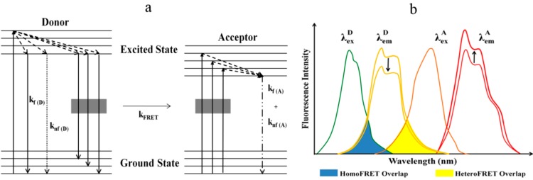
Figure 1
( a ) The figure shows the Jablonski diagram demonstrating mechanism of Fu00f6rster Resonance Energy Transfer (FRET). On absorption of energy, electrons in both donor and acceptor are excited from the...
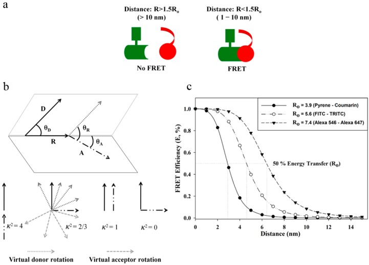
Figure 2
( a ) A schematic representation of FRET between two molecules; ( b ) The orientation of emission dipole moment of donor and absorption dipole moment of acceptor is illustrated in this figure. u201cRu...
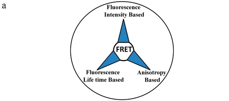
Figure 3
( a ) Schematic representation of types of FRET measurements based on photophysical features; and ( b ) This figure illustrates the effect of heteroFRET and homoFRET on fluorescence intensity ( left p...
Figure images are served from the NIH/NLM PubMed Central Open Access Subset or Europe PMC; copyright remains with the publishers and authors.
💬 Discussion
0 commentsNo comments yet. Be the first to start a discussion!
Leave a Comment