Abstract
AbstractHigh-speed three-dimensional (3D) intravital imaging in animals is useful for studying transient subcellular interactions and functions in health and disease. Light-field microscopy (LFM) provides a computational solution for snapshot 3D imaging with low phototoxicity but is restricted by low resolution and reconstruction artifacts induced by optical aberrations, motion and noise. Here, we propose virtual-scanning LFM (VsLFM), a physics-based deep learning framework to increase the resolution of LFM up to the diffraction limit within a snapshot. By constructing a 40 GB high-resolution scanning LFM dataset across different species, we exploit physical priors between phase-correlated angular views to address the frequency aliasing problem. This enables us to bypass hardware scanning and associated motion artifacts. Here, we show that VsLFM achieves ultrafast 3D imaging of diverse processes such as the beating heart in embryonic zebrafish, voltage activity in Drosophila brains and neutrophil migration in the mouse liver at up to 500 volumes per second.
🔬 Techniques
🔭 Microscopes
🧬 Organisms
💻 Software
✨ Fluorophores
🧪 Sample Preparation
🔬 Cell Lines
🏭 Microscope Brands
🧪 Reagent Suppliers
🔴 Lasers
📷 Detectors
💻 Software Details
🏛️ Research Organizations (ROR)
Affiliated research institutions:
📋 Methods
VsLFM set-up and data collection
The inverted sLFM optical system was built in accordance with our previous research 20 . A standard inverted fluorescence microscope (Zeiss, Observer Z1) was used as a basic imaging module, configured with a ×63/1.4 NA oil-immersion objective (Zeiss Plan-Apochromat ×63/1.4 NA Oil M27) and a ×20/0.5 NA air-immersion objective (Zeiss EC Plan-Neofluar ×20/0.5 NA M27) for different experiment requirements. A microlens array with the pitch size of 100 μm and focal length of 2,100 μm modulated the emission light into a 4D light field, with a 2D galvo system to shift the image plane periodically at high speed. Each microlens covered 13 × 13 sensor pixels for angular sampling. Multi-channel lasers (Coherent OBIS 405/488/561/640) and a scientific camera (Andor Zyla 4.2 Plus PCIE) were used for fluorescence excitation and data collection. All hardware synchronization of the system was carried out using a National Instruments (NI) control box (NI USB-6363) and LabVIEW software (2019 version), which were integrated in an acquisition graphical user interface named sLFdriver, as described in the published protocol 45 . To construct the training dataset, scanning light-field images with the scanning period of 3 × 3 (2,048 × 2,048 pixels each) were captured by sLFM. Then, the light-field image taken in the middle of the series was extracted as the paired low-resolution light-field image. Next, a pixel-realignment algorithm was performed on the single light-field image and scanning light-field images to yield the paired low-resolution and high-resolution spatial–angular views, which were regarded as the input and target for network training. For example, in the inverted sLFM system, the low-resolution spatial–angular views consist of 153 × 153 spatial pixels and 13 × 13 angular pixels, and the high-resolution spatial–angular views consist of 459 × 459 spatial pixels and 13 × 13 angular pixels, which are determined by the parameters of the microlens array and camera. We also constructed an upright sLFM system for imaging voltage activities in Drosophila brains, configured with a ×25/1.05 NA water-immersion objective (Olympus XLPLN25XWMP2) and a high-speed scientific camera (Teledyne Photometrics Kinetix). In the implementation of the upright system, a customized microlens array with a pitch size of 136.5 μm and a focal length of 2,800 μm was used to cover 21 × 21 angular pixels for a large axial coverage. During the Drosophila experiment, the camera pixel region was set to 2,000 × 2,000, with LFM data containing 91 × 91 spatial pixels and 21 × 21 angular pixels, and sLFM data containing 273 × 273 spatial pixels and 21 × 21 angular pixels. When capturing test data for VsLFM, the 2D galvo was set to its offset voltage and kept stable as in traditional LFM. Then the system captured single-frame or time-lapse light-field data, and further realigned them into low-resolution spatial–angular views, of which spatial resolution would be improved by the virtual-scanning framework. Each frame of VsLFM was collected within a snapshot. For intuitive comparisons between VsLFM and sLFM, the unscanned light-field images were directly extracted from scanning light-field images. The snapshot images were used to derive the results of VsLFM, and the sLFM results were used as the paired ground truth for performance comparison. The data used in testing were not involved in network training. Detailed imaging conditions for all of the fluorescence experiments in this study, including the fluorescent label, exposure time, excitation power, volume rate and objective, are listed in Supplementary Table 2 .
Show full methods section
VsLFM set-up and data collection
The inverted sLFM optical system was built in accordance with our previous research 20 . A standard inverted fluorescence microscope (Zeiss, Observer Z1) was used as a basic imaging module, configured with a ×63/1.4 NA oil-immersion objective (Zeiss Plan-Apochromat ×63/1.4 NA Oil M27) and a ×20/0.5 NA air-immersion objective (Zeiss EC Plan-Neofluar ×20/0.5 NA M27) for different experiment requirements. A microlens array with the pitch size of 100 μm and focal length of 2,100 μm modulated the emission light into a 4D light field, with a 2D galvo system to shift the image plane periodically at high speed. Each microlens covered 13 × 13 sensor pixels for angular sampling. Multi-channel lasers (Coherent OBIS 405/488/561/640) and a scientific camera (Andor Zyla 4.2 Plus PCIE) were used for fluorescence excitation and data collection. All hardware synchronization of the system was carried out using a National Instruments (NI) control box (NI USB-6363) and LabVIEW software (2019 version), which were integrated in an acquisition graphical user interface named sLFdriver, as described in the published protocol 45 . To construct the training dataset, scanning light-field images with the scanning period of 3 × 3 (2,048 × 2,048 pixels each) were captured by sLFM. Then, the light-field image taken in the middle of the series was extracted as the paired low-resolution light-field image. Next, a pixel-realignment algorithm was performed on the single light-field image and scanning light-field images to yield the paired low-resolution and high-resolution spatial–angular views, which were regarded as the input and target for network training. For example, in the inverted sLFM system, the low-resolution spatial–angular views consist of 153 × 153 spatial pixels and 13 × 13 angular pixels, and the high-resolution spatial–angular views consist of 459 × 459 spatial pixels and 13 × 13 angular pixels, which are determined by the parameters of the microlens array and camera. We also constructed an upright sLFM system for imaging voltage activities in Drosophila brains, configured with a ×25/1.05 NA water-immersion objective (Olympus XLPLN25XWMP2) and a high-speed scientific camera (Teledyne Photometrics Kinetix). In the implementation of the upright system, a customized microlens array with a pitch size of 136.5 μm and a focal length of 2,800 μm was used to cover 21 × 21 angular pixels for a large axial coverage. During the Drosophila experiment, the camera pixel region was set to 2,000 × 2,000, with LFM data containing 91 × 91 spatial pixels and 21 × 21 angular pixels, and sLFM data containing 273 × 273 spatial pixels and 21 × 21 angular pixels. When capturing test data for VsLFM, the 2D galvo was set to its offset voltage and kept stable as in traditional LFM. Then the system captured single-frame or time-lapse light-field data, and further realigned them into low-resolution spatial–angular views, of which spatial resolution would be improved by the virtual-scanning framework. Each frame of VsLFM was collected within a snapshot. For intuitive comparisons between VsLFM and sLFM, the unscanned light-field images were directly extracted from scanning light-field images. The snapshot images were used to derive the results of VsLFM, and the sLFM results were used as the paired ground truth for performance comparison. The data used in testing were not involved in network training. Detailed imaging conditions for all of the fluorescence experiments in this study, including the fluorescent label, exposure time, excitation power, volume rate and objective, are listed in Supplementary Table 2 .
Virtual-scanning network
In our proposed Vs-Net, the input is a 3D tensor of low-resolution spatial–angular views (rearranged into the form of height × width × angle), while the output is a 3D tensor of high-resolution spatial–angular views. For the preprocessing of data captured by the inverted system, the training dataset was partitioned into small patches with the input size of 25 × 25 × 169 pixels, and the output and target size of 75 × 75 × 169 pixels. The input and corresponding target data were normalized by the average value of maximum intensities from different time-lapse data. An overview of Vs-Net architecture is given in Supplementary Fig. 2a and the detailed network parameters for each layer are listed in Supplementary Table 1 . In our implementation, Vs-Net emphasizes the spatial–angular feature and angular–mixed feature on the basis of a global residual network containing feature extraction, interaction and fusion modules 40 . The input spatial–angular views (size of 25 × 25 × 169 pixels, height × width × angle) are first fed into the feature extractor to generate spatial–angular features (size of 169 × 25 × 25 × C pixels, angle × height × width × channel), light-field features (size of 325 × 325 × C pixels, height × width × channel) and angular–mixed features (size of 25 × 25 × C pixels, height × width × channel), where C denotes the channel number of 2D convolution layers and is usually set to 64. The spatial–angular feature is extracted to better consider the phase correlation induced by the diffraction effect of the small microlens aperture and the disparity between different angular views in LFM, which is much larger than that used in macroscale light-field photography due to the large collection angle of the objective lens. The light-field feature is generated for comprehensive consideration of the angular information at different local spatial regions. The angular–mixed feature, weighted by multiple angular views, is used to reinforce the fidelity of fine structures under strong noise conditions. We use only linear operations to reshape and decouple the input into features of these three domains, leaving non-linear activation and deeper layers to the subsequent interaction and fusion stage to obtain more expressive features. Note that the linear operations such as pixel alignment and dilated convolution should have the appropriate parameters associated with the LFM configuration and data structure. The three features are then passed through the feature interaction and fusion modules to enable multiple information interaction and integration. The detailed structures of the interaction and fusion modules are shown in Supplementary Fig. 2b . The light-field interaction module plays the major role in enhancing the spatial resolution, while the spatial–angular feature and the angular–mixed feature are considered as complementary information and interact with the light-field feature for spatial super-resolution, to provide sufficient consideration of phase correlation between different angles and to reinforce the fidelity of fine structures under strong noises. During the learning process, the light-field feature is interactively fused with the spatial–angular feature and the angular–mixed feature in the spatial–angular interaction module and the angular–mixed interaction module, respectively. We apply a local residual connection in the output features of the aforementioned interaction modules to fully extract the features. The ablation study demonstrates the effective collaboration of the interaction modules and verifies the functions of the three features (Supplementary Fig. 3 ). The feature interaction modules are followed by a K cascade and concatenation module, where K denotes the cascaded number, usually set to 4. Next, the concatenated interacted spatial–angular feature (size of 169 × 25 × 25 × K·C pixels, angle × height × width × K-fold channels) and angular–mixed feature (size of 25 × 25 × K·C pixels), are realigned into the light-field domain and subsequently squeezed into C channels before concatenating with K light-field features (size of 325 × 325 × K·C pixels), to yield the fully concatenated interacted features (size of 325 × 325 × (K + 2)·C pixels). The concatenated interacted features are fused by a 1 × 1 convolution layer and a leaky rectified linear unit (Leaky ReLU) layer to generate the fused light-field feature (size of 325 × 325 × C pixels). Last, the fused features are fed into the upsampling module with a pixel shuffle to be scaled up by 3 to produce the high-resolution spatial–angular views (size of 75 × 75 × 169 pixels, height × width × angle). In addition, a global residual connection is used by adding the output and the upsampled input with bicubic interpolation, to fully recover the high-frequency details and speed up the convergence. For network training we typically used 5,000 paired spatial–angular patches of the same dataset, and it usually took approximately 40 epochs for network convergence. Considering the inherent sparsity of fluorescent specimens 52 , the pixel-wise mean absolute error (L1-norm error) is adopted as the loss function, which could be expressed as: documentclass[12pt]{minimal} usepackage{amsmath} usepackage{wasysym} usepackage{amsfonts} usepackage{amssymb} usepackage{amsbsy} usepackage{mathrsfs} usepackage{upgreek} setlength{oddsidemargin}{-69pt} begin{document}$${mathrm{loss}} = left| {X - Y} right|_1,$$end{document} loss = X − Y 1 , where X denotes the ground truth of spatial–angular views and Y denotes the output spatial–angular views. The parameters of the Adam optimizer were set to β 1 = 0.9, β 2 = 0.999. The learning rate was initialized to 2 × 10 −4 and then decreased by a factor of 0.5 for every 10 epochs during the training process. Vs-Net works well for different types of data and has the robust flexibility of input size. After the network is trained, it can be applied to specimens from different organism. For the inference process, the input data with the size of 153 × 153 × 169 pixels are first partitioned into nine partially overlapping patches with the size of 69 × 69 × 169 pixels, and then transformed to nine high-resolution outputs with the size of 207 × 207 × 169 pixels, using sigmoid-based image fusion 53 to generate the final output with the size of 459 × 459 × 169 pixels. Finally, the output spatial–angular views are used to obtain the high-resolution volume by iterative tomography with DAO, which has been described in the previous work 20 . The validity of Vs-Net has been verified in extensive fluorescence specimens including fluorescent beads, living cells with mitochondria and membrane labeling, blood cells in zebrafish larvae, immune cells in mouse livers, and voltage indicators in Drosophila . To validate the considerable scalability and generalization capability of Vs-Net, both numerical simulations and biological experiments were performed. First, we performed a generalization test on cross-channel tasks, in which the mitochondria channel and membrane channel in L929 cells were mutually trained and predicted (Fig. 4a–c ). Second, a Vs-Net model that was pre-trained on mouse liver data with vessel and neutrophil labeling under a ×63/1.4 NA oil-immersion objective, performed well on highly dynamic membrane and blood cells in a living zebrafish larva, which were captured by another air-immersion objective (Fig. 4d–g and Supplementary Fig. 15 ). Third, synthetic specimens of beads and tubulins, which have great morphological differences, were selected for cross-sample and transfer learning experiments (Supplementary Figs. 14 and 19 ). The Vs-Net can work on data captured by LFM with different kinds of microlens arrays through slight network modifications. To enable Vs-Net to accommodate data with different angular pixels, we need to modify the parameter of angular numbers of the network, while the main architecture of the network remains the same as before. To verify it, we set up an upright system, in which another microlense array with the pitch size of 136.5 μm and focal length of 2,800 μm was used. The data obtained by the upright system have 21 × 21 angular views, whereby the input size of the training dataset patches is 25 × 25 × 441 pixels (height × width × angle) and the output and target sizes are 75 × 75 × 441 pixels. Correspondingly, the spatial–angular feature has the size of 441 × 25 × 25 × C pixels (angle × height × width × channel), the light-field feature has the size of 525 × 525 × C pixels (height × width × channel) and the angular–mixed feature has the size of 25 × 25 × C pixels (height × width × channel), where C is usually set to 64 or 32, dependent on the GPU (graphics processing unit) memory. After network training, the test data can be enhanced by Vs-Net. The Drosophila data in Fig. 6 were processed by the Vs-Net with 21 × 21 angular views as input. The VsLFM results have comparable resolution to those of sLFM when there were no motion artifacts. The network was implemented on a PyTorch platform with two NVIDIA RTX 2080 Ti GPUs. The whole training process for 40 epochs on a typical training set (approximately 5,000 pairs) took approximately 16 h, and inference and post-processing on one whole-FOV light-field image took approximately 5 s for a spatial–angular image size of 459 × 459 × 169 pixels. Training and inference time can be further reduced by using more powerful GPUs. To maximize its accessibility, we have released Vs-Net codes and corresponding 3D reconstruction scripts with demonstration data to promote interdisciplinary research.
Comparison with previous methods
We compared our method with the previous methods, such as traditional LFM, sLFM, CARE, DFCAN and DFGAN, LF-InterNet, LF-DFnet, VCD-Net and HyLFM-Net. All traditional LFM results used in this work were reconstructed using phase-space deconvolution with a simple bicubic interpolation applied on the low-resolution spatial–angular views 25 . All sLFM results were acquired as described in the original study 20 , and all in vivo biological results were obtained with DAO, but for simplicity, DAO is no longer specified in the texts. For comparison with CARE 35 , DFCAN 37 and DFGAN 37 , we adopted two training strategies for comprehensive evaluations. First, we trained the networks on the same spatial–angular views used in Vs-Net, which were split into two stacks of images consisting of low-resolution and high-resolution pairs (Supplementary Figs. 4 and 5 ). For CARE, we used the bicubic interpolation to upsample the low-resolution images by a factor of 3 and cropped them into patches with 128 × 128 pixels (height × width) as input, and the corresponding high-resolution images were also cropped into patches with 128 × 128 pixels as targets. For the training of DFCAN and DFGAN, the low-resolution data were cropped into patches with 64 × 64 pixels as input, and high-resolution resolution data were cropped into patches with 192 × 192 pixels as targets. The scale factor was adjusted to 3. The training process took approximately 10 h for CARE, 12 h for DFCAN and 18 h for DFGAN on a single NVIDIA RTX 2080 Ti GPU for convergence. After network inference, the output images were re-stacked as spatial–angular views according to their angular positions, and the final whole-FOV results were obtained with the same sigmoid-based image fusion used in Vs-Net. The results of the comparisons are shown in Supplementary Figs. 4 and 5 . Second, we also trained the networks based on the reconstructed volumes of LFM and sLFM for comparison (Supplementary Fig. 6 ). In this case, the data pairs consisted of the low-resolution volumes of LFM (with the size of 1,989 × 1,989 × 101 pixels, height × width × depth) and the high-resolution volumes of sLFM (with the size of 1,989 × 1,989 × 101 pixels). For CARE, the data pairs were cropped into 3D patches with the size of 128 × 128 × 16 pixels for training. For DFCAN and DFGAN, which are designed for SISR tasks, the 3D volume pairs were segmented as a stack of images. The input low-resolution data were downsampled by a factor of 3 and cropped into patches with the size of 128 × 128 pixels, while high-resolution targets were cropped into patches with the size of 384 × 384 pixels. The training processes of CARE, DFCAN and DFGAN were performed on a single NVIDIA RTX 2080 Ti GPU, which took approximately 20 h for CARE, 25 h for DFCAN and 40 h for DFGAN for convergence. After network inference the outputs were stitched using sigmoid-based image fusion working in 3D or 2D space. LF-InterNet 40 requires raw light-field images as input and high-resolution spatial–angular images as targets, while LF-DFnet 41 requires tiled low-resolution spatial–angular images as input and tiled high-resolution spatial–angular images as targets. The training inputs used for Vs-Net with the size of 25 × 25 × 169 pixels (height × width × angle) were transformed to light-field images with the size of 325 × 325 pixels (height × width) for LF-InterNet as input, and tiled to images with the size of 325 × 325 pixels (height × width) for LF-DFnet as input. Correspondingly, the high-resolution spatial–angular images from the Vs-Net dataset were tiled to images with the size of 975 × 975 pixels (height × width) as targets for both LF-InterNet and LF-DFnet. The tiling operation stitches images from different angles into a 2D image according to their angular positions in the way of a montage. The whole training process of LF-InterNet and LF-DFnet took approximately 14 h and 20 h, respectively, on a single NVIDIA RTX 2080 Ti GPU for convergence. After network inference the outputs were rearranged according to the spatial–angular domain, and stitched by the same sigmoid-based image fusion used in Vs-Net. The results are compared in Supplementary Figs. 4 and 5 . VCD-Net 31 and HyLFM-Net 32 require light-field images as input data and corresponding confocal or light-sheet volumes as targets, to train fully supervised models. However, the target volumes are difficult to acquire if using a simple LFM or sLFM system. To compare VsLFM with VCD-Net and HyLFM-Net, we first conducted numerical simulations in which the required confocal or light-sheet volumes could be replaced by the original synthetic volumes, to quantitatively evaluate their performance in complicated environments (Fig. 3 and Supplementary Fig. 14 ). To mimic the practical situations for fair comparison between different methods, we trained Vs-Net, VCD-Net and HyLFM-Net in the same ideal imaging conditions, and performed network inferences in multiple complicated scenes. We also compared VsLFM with VCD-Net and HyLFM-Net on experimental data (Figs. 2 , 4 and Supplementary Fig. 7 ). Given that the confocal and light-sheet modules are difficult to integrate into the sLFM system, the high-resolution volumes acquired by sLFM with 3D reconstruction were used as training labels. The VCD-Net and HyLFM-Net results in Figs. 2 – 4 and Supplementary Figs. 7 , 14 were obtained using open-source codes in previous studies 31 , 32 , and the corresponding parameter of angle number was adjusted to make it suitable for our system implementations. Specifically, the number of input channels of VCD-Net and HyLFM-Net was modified to 169, and a bicubic interpolation layer was attached to the end of each network to match the output volume size of the target. The input data are the same as that used in Vs-Net, with the size of 153 × 153 × 169 pixels. For network training we randomly cropped out small input patches with the size of 40 × 40 × 169 pixels (for HyLFM-Net) and 64 × 64 × 169 pixels (for VCD-Net), as well as the corresponding volume regions, to create data pairs. The networks required to be trained for around 200 epochs for convergence. For network inference, partially overlapped patches with the size of 80 × 80 × 169 pixels (for HyLFM-Net) and 64 × 64 × 169 pixels (for VCD-Net) were cropped from input data. The same sigmoid-based image fusion used in Vs-Net was adopted to stitch the output sub-volumes into whole-FOV volumes. The whole training process of VCD-Net and HyLFM-Net took approximately 32 h, and the inference time for one whole-FOV frame took approximately 3 s for VCD-Net and 7 s for HyLFM-Net. The network training and inference were done on a single NVIDIA RTX 2080 Ti GPU. We also develop a new end-to-end network, termed HyLFM-A-Net, which imposes channel attention 48 on the existing HyLFM-Net, to further increase the computational efficiency of 3D reconstruction for VsLFM. HyLFM-A-Net is designed to accommodate high-resolution angular views with 3 × 3 scanning as input, with full-sampled high-resolution volumes as labels. The detailed architecture of HyLFM-A-Net is shown in Supplementary Fig. 17a,b . The output of Vs-Net prediction was used directly for the input of HyLFM-A-Net, with a patch size of 120 × 120 × 169 pixels (height × width × angle), while the target data consisted of the reconstruction results by iterative tomography with the size of 520 × 520 × 101 pixels (height × width × depth). 2D convolutions with channel attention were followed to extract features with a size of 120 × 120 × 64 pixels (height × width × channel), then two subpixel convolutions were used to recover the spatial resolution into 480 × 480 × 64 pixels. Another two convolutions with channel attention were used to adjust the feature channels into the size of 808, which was eightfold the output depth. We rearranged the 2D features into 3D features with a size of 480 × 480 × 8 × 101 pixels (height × width × channel × depth) and used 3D convolutions to fuse the features into 480 × 480 × 101 pixels (height × width × depth). A bicubic interpolation layer was attached to the end of the network to match the volume size of 520 × 520 × 101 pixels for supervision. A detailed comparison of HyLFM-Net and HyLFM-A-Net is given in Supplementary Fig. 17f . The channel size and feature size of HyLFM-Net and HyLFM-A-Net had been adjusted to our LFM set-up. HyLFM-A-Net follows the concept of HyLFM-Net, in which the depth dimension is rearranged using 2D channels that are integer multiples of the depth, and then the multiple is considered as the channel of 3D features. Attention operators were applied on 2D layers before rearrangement. For HyLFM-Net, the affine layer was used when it was trained with light-sheet continuous supervision, but when trained with sLFM reconstruction, the affine layer was removed. We trained 400 epochs in 14 h on a single NVIDIA RTX 3090 GPU for convergence. During inference, the Vs-Net output with the size of 459 × 459 × 169 pixels was cropped into four overlapping patches with a size of 237 × 237 × 169 pixels, and the same sigmoid-based image fusion mentioned above was used for volume stitching. The whole inference time of HyLFM-A-Net for a single volume with a size of 1,989 × 1,989 × 101 pixels is approximately 6 s, while 11 s in total is required with Vs-Net inference involved, which is comparable to the inference time of HyLFM-Net. HyLFM-A-Net achieves a similar performance to that of 3D deconvolution in the imaging of living cells, with reduced computation costs at the cost of aberration robustness (Supplementary Fig. 17c – e ). All of the deep learning networks used for comparison were trained on the same dataset as that used in VsLFM.
Beads preparation and resolution characterization
For the fluorescent beads preparation, 1 ml 100-nm-diameter fluorescent beads (Thermo Fisher TetraSpeck Microspheres, T7279) were diluted with 100 ml pure water at room temperature to produce diluted fluorescent beads. Then 10 mg ml −1 diluted agarose was produced by mixing 1,000 mg pure agarose (Thermo Fisher UltraPure Low Melting Point Agarose, 16520100) with 100 ml pure water at 80 °C. When diluted agarose cooled to 40 °C, 1 ml diluted agarose and 1 μl diluted fluorescent beads were mixed well. Next, a 200 μl mixture of beads and agarose was put into a 35 mm dish (Thermo Fisher Nunc glass bottom dish, 150682) and left for 30 min to solidify to produce a uniform 3D distribution of beads. A ×63/1.4 NA oil-immersion objective was selected to verify the high-resolution capability of VsLFM. The temperature of the imaging environment was controlled at around 27 °C. For quantitative resolution analysis, the FWHM was calculated by measuring the intensity distributions of the reconstructed cross-section planes of the beads laterally and axially using a Gaussian fit. The calculation was conducted with MATLAB software on the results of LFM, VsLFM and sLFM, respectively. The FWHMs are presented as bar plots, in which the mean values and the standard deviations indicate the distribution of spatial resolution at different axial positions.
Living L929 cell imaging
L929 cells were cultured in DMEM (Gibco) medium supplemented with 10% FBS (Biological Industries), 2 mM GlutaMAX and 100 U ml −1 penicillin–streptomycin in 5% CO 2 at 37 °C. The PiggyBac Transposon Vector System and Vigofect were used for cell transfection to generate L929 TSPAN4-mCherry and TOM20-GFP stable cell lines 54 . L929 cells were cultured on a fibronectin-coated confocal dish and in DMEM (no phenol red) (Gibco) medium for imaging. During imaging, a microscope incubator system (Tokai Hit, INUF-IX3D-F1) was used to maintain the environmental conditions of 37 °C and a CO 2 concentration of 5%.
Zebrafish imaging
For imaging of zebrafish embryos, the cultured embryos were injected with 300 pg Tspan4a -EGFP messenger RNA (synthesized in vitro with mMessage mMachine T7 kit, Ambion, AM1344) in one cell at the 16-cell stage. Then the embryos were mounted in 1% low-melting-point agarose. During imaging, a ×63/1.4 NA oil-immersion objective was used, and the environment temperature was set at around 27 °C. For imaging of blood flow dynamics in zebrafish larvae, Tg ( flk:EGFP ; gata1:DsRed ) transgenic zebrafish embryos were collected and cultured in Holtfreter’s solution at 28.5 °C. At 3–4 days postfertilization the zebrafish larvae were anesthetized using ethyl 3-aminobenzoate methanesulfonate salt (100 mg l −1 ) and embedded in 1% low-melting-point agarose in 35 mm confocal dishes (Thermo Fisher Nunc glass bottom dish, 150682) for in vivo imaging. During imaging, a ×20/0.5 NA air-immersion objective was selected to cover an FOV of 600 × 600 μm 2 , and the environmental temperature was set at around 27 °C. Mouse experiments The mice used in this project were male and wild type (C57BL6/J, around 7–8 weeks). Mice were housed with food and water available ad libitum under a 12 h light–dark cycle at 22 °C with a relative air humidity of ~50%. For the mice labeled with neutrophils and vessels, 1 μg Ly6G/Ly6C monoclonal antibody (PE-Cyanine7, eBioscience, 25-4317-82), 3 μg AF647-WGA (Alexa Fluor 647 Conjugate, Thermo Fisher, P21462 ) and 100 μl PBS were injected i.v. After 30 min, Avertin (350 mg kg −1 ) was injected i.p. into the mice for anesthetization. After 20 min, the deeply anesthetized mice were dissected to expose the living liver on a home-made holder with a 170-μm-thick coverslip for intravital imaging. A ×63/1.4 NA oil-immersion objective was selected to capture subcellular dynamics. During the intravital imaging, a 37 °C body temperature maintenance instrument (ThermoStar Homeothermic Monitoring System, RWD) was launched to maintain the mouse in the native physiological state. Drosophila experiments Drosophila strains ( MB065B-GAL4 > 20×UAS-pAce ) were provided by the Schnitzer laboratory at Stanford University and the Zhong laboratory at Tsinghua University. The Drosophila used in our experiments were female at 3–7 days and raised on the standard cornmeal agar media with a 12 h light–dark cycle at 25 °C. Based on the protocol described previously 55 , Drosophila were anesthetized on ice and mounted on a 3D-printed plastic disk with free movement of the legs. Then, the posterior head capsule was opened using sharp forceps (5SF, Dumont) in carbonated (95% O 2 , 5% CO 2 ) buffer solution with a pH of 7.3 and an osmolarity of 275 mosM. Next, the air sacs, tracheas and M16 muscle were removed to minimize brain movement 56 . Ultraviolet glue was also added around the proboscis. After the surgery, Drosophila were placed under the objective lens for imaging of voltage transients in sparsely labeled neurons. For neural recording of the response to odor stimulus, 3% benzaldehyde was fed in a 5 s on–5 s off cycle.
Neural extraction and analysis
For neural analysis of Drosophila data, we manually selected several regions of interest (ROIs) as shown in Fig. 6 . The temporal traces of neural activity were calculated as ΔF/F 0 = ( F–F 0 ) /F 0 , where F is the averaged intensity of the ROI and F 0 is the baseline intensity. F 0 was calculated as the mean fluorescence in the ROI averaged over the entire time series. The neural spikes were identified as the local peaks that rose above a threshold value (2% for VsLFM results and 1.2% for sLFM results) after the median-filtered (40 ms window) version was subtracted from the ΔF/F 0 curve, and visualized as flashes of light in Supplementary Video 6 . Each identified spike was temporally aligned to the time at which its peak value of ΔF/F 0 occurred, to generate the average spike waveforms. The FWHM of each spike was calculated by measuring the intensity distribution of the spike temporal trace using a Gaussian fit. The amplitude of each spike was calculated as the absolute value of the peak. The peak time map was extracted from a single peak in the captured movie, in line with the previously reported method 57 . Specifically, we first applied a spatial Gaussian filter with a standard deviation of 9 voxels and a wavelet-based denoising method to each voxel independently. Then we fitted the filtered data with a quadratic spline interpolation. Finally, we used the threshold crossing time on the rising edge as the peak time of a specific voxel to generate the whole peak time map. The video of subframe propagation was made based on the peak time map. The firing rate was calculated as the number of spikes per second in the resting or stimulated state, and the curve was obtained with a 1 s temporal sliding window.
Ethics statement
This work complies with all relevant ethics regulations for animal research and testing. All experimental procedures were performed with ethics approval from the Animal Care and Use Committee (IACUC) of Tsinghua University.
Data analysis
All data processing and analyses were performed with customized MATLAB (MathWorks, MATLAB 2018b) scripts and Python (v3.7) scripts. The data collection and hardware control were performed with LABVIEW (2019 version) and our previously developed graphical user interface (sLFdriver 45 , v2.0). The 3D volumes of Drosophila brain in Fig. 6 were rendered using Imaris (v9.0.1). The 3D rendering of the volumes in the supplementary videos was carried out using Voltex modules in Amira (Thermo Fisher Scientific, Amira 2019). The 3D tracking of blood cells in the vessels of the zebrafish larvae and the neutrophil in the vessels of mouse liver was carried out automatically using Imaris (v9.0.1).
Performance metrics
We chose signal-to-noise ratio, structural similarity (SSIM) and cut-off frequency ( k c ) 58 to quantitatively evaluate the capability of VsLFM. Synthetic volumes or sLFM results were regarded as ground truth, as described in the Figure legends. The signal-to-noise ratio is calculated by the following formula: documentclass[12pt]{minimal} usepackage{amsmath} usepackage{wasysym} usepackage{amsfonts} usepackage{amssymb} usepackage{amsbsy} usepackage{mathrsfs} usepackage{upgreek} setlength{oddsidemargin}{-69pt} begin{document}$${mathrm{SNR}} = 10log _{10}frac{{left| X right|_2^2}}{{left| {X - Y} right|_2^2}},$$end{document} SNR = 1 0 log 10 X 2 2 X − Y 2 2 , where X represents the ground truth and Y represents the corresponding reconstructed results. SSIM is calculated by the following formula: documentclass[12pt]{minimal} usepackage{amsmath} usepackage{wasysym} usepackage{amsfonts} usepackage{amssymb} usepackage{amsbsy} usepackage{mathrsfs} usepackage{upgreek} setlength{oddsidemargin}{-69pt} begin{document}$${mathrm{SSIM}} = frac{{left( {2{mu} _{X}{mu} _{Y} + left( {0.01 cdot L} right)^2} right)left({2{sigma}_{XY} + left( {0.03 cdot L} right)^2} right)}}{{left( {mu _X^2 + mu _Y^2 + left( {0.01 cdot L} right)^2} right)left( {sigma _X^2 + sigma _Y^2 + left( {0.03 cdot L} right)^2} right)}},$$end{document} SSIM = 2 μ X μ Y + 0.01 ⋅ L 2 2 σ X Y + 0.03 ⋅ L 2 μ X 2 + μ Y 2 + 0.01 ⋅ L 2 σ X 2 + σ Y 2 + 0.03 ⋅ L 2 , where X and Y represent the signals, µ X and µ Y represent the average values of each signal, σ X and σ Y represent the corresponding standard deviations of each signal, and σ XY represents the cross-covariance for X and Y . The dynamic-range value L in this work is 1 after the data were normalized to single-precision floating-point numbers. The SSIM indices were calculated on 2D images (Supplementary Figs. 3h , 4b , 8b , 8e , 9d , 18d ) or 3D images (Fig. 3f and Supplementary Figs. 4a , 19b ), according to different evaluation requirements. For SSIM calculation on 2D images, we calculated the local SSIM maps with multiple (sliding) 2D local Gaussian windows (with the size of 11 × 11 and standard deviation of 1.5) and averaged them to produce the SSIM metric. For SSIM calculation on 3D images, we first reshaped the 4D angular views (height × width × 13 × 13) into a 3D form (height × width × 169). The 169 angles were arranged based on their spatial proximity. Then local SSIM maps were computed in multiple (sliding) 3D local Gaussian windows (with the size of 11 × 11 × 11 and standard deviation of 1.5) of the 3D image. Finally, the mean value of the local SSIM maps was returned as the SSIM metric. In practice, the calculations were conducted using the built-in ssim.m function in MATLAB R2018b. For decorrelation analysis of images 58 , the cross-correlation coefficient is calculated by the following formula: documentclass[12pt]{minimal} usepackage{amsmath} usepackage{wasysym} usepackage{amsfonts} usepackage{amssymb} usepackage{amsbsy} usepackage{mathrsfs} usepackage{upgreek} setlength{oddsidemargin}{-69pt} begin{document}$$dleft( r right) = frac{{{int} {{Re} left{ {Ileft( {{{boldsymbol{k}}}} right)I_n^ ast left( {{{boldsymbol{k}}}} right)Mleft( {{{{boldsymbol{k}}}};r} right)} right}dk_xdk_y} }}{{sqrt {{int} {left| {Ileft( {{{boldsymbol{k}}}} right)} right|^2} dk_xdk_y{int} {left| {I_nleft( {{{boldsymbol{k}}}} right)Mleft( {{{{boldsymbol{k}}}};r} right)} right|^2dk_xdk_y} } }},$$end{document} d r = ∫ ℜ I k I n * k M k ; r d k x d k y ∫ I k 2 d k x d k y ∫ I n k M k ; r 2 d k x d k y , where I ( k ) denotes the Fourier transform of the input image, I n ( k ) denotes the normalized form of I ( k ), k = ( k x , k y ) denotes the Fourier space coordinates and M ( k ;r ) denotes the binary mask of radius r . Then the cut-off frequency ( k c ) is calculated by the following formula: documentclass[12pt]{minimal} usepackage{amsmath} usepackage{wasysym} usepackage{amsfonts} usepackage{amssymb} usepackage{amsbsy} usepackage{mathrsfs} usepackage{upgreek} setlength{oddsidemargin}{-69pt} begin{document}$$k_c = max left{ {r_i} right},$$end{document} k c = max r i , where r i denotes the radius of the binary mask, corresponding to the frequency of the highest peak. We also used the Pearson correlation coefficient ( R ) to evaluate the similarity between the ground truth and the results by different methods. R is calculated by the following formula: documentclass[12pt]{minimal} usepackage{amsmath} usepackage{wasysym} usepackage{amsfonts} usepackage{amssymb} usepackage{amsbsy} usepackage{mathrsfs} usepackage{upgreek} setlength{oddsidemargin}{-69pt} begin{document}$$R = frac{{Eleft[ {left( {X - mu _X} right)left( {Y - mu _Y} right)} right]}}{{sigma _Xsigma _Y}},$$end{document} R = E X − μ X Y − μ Y σ X σ Y , where X and Y denote the signals, µ X and µ Y represent mean values of each signal, σ X and σ Y denote the corresponding standard deviations of each signal, and E [·] denotes the expectation. For quantitative analysis on Fourier spectra (Fig. 4e ), the Fourier ring correlation (FRC) were applied as described in the original paper 43 . In the calculation of the FRC curve, the threshold was set to 1/7 ≈ 0.143 for the cut-off frequency.
Statistics and reproducibility
Biological data shown in Figs. 2 , 4 , 5 , 6 and Supplementary Figs. 4 , 5 , 6 , 15 , 16 are representative of n = 6 experiments. Biological data shown in Supplementary Figs. 9 and 13 are representative of n = 12 experiments. Simulated data shown in Fig. 3 and Supplementary Figs. 10 , 12 are representative of n = 17 experiments. Simulated data shown in Supplementary Figs. 1 , 8 , 11 , 14 , 17 , 18 , 19 are representative of n = 20 experiments. Reporting summary Further information on research design is available in the Nature Portfolio Reporting Summary linked to this article.
Comparison with previous methods
We compared our method with the previous methods, such as traditional LFM, sLFM, CARE, DFCAN and DFGAN, LF-InterNet, LF-DFnet, VCD-Net and HyLFM-Net. All traditional LFM results used in this work were reconstructed using phase-space deconvolution with a simple bicubic interpolation applied on the low-resolution spatial–angular views 25 . All sLFM results were acquired as described in the original study 20 , and all in vivo biological results were obtained with DAO, but for simplicity, DAO is no longer specified in the texts. For comparison with CARE 35 , DFCAN 37 and DFGAN 37 , we adopted two training strategies for comprehensive evaluations. First, we trained the networks on the same spatial–angular views used in Vs-Net, which were split into two stacks of images consisting of low-resolution and high-resolution pairs (Supplementary Figs. 4 and 5 ). For CARE, we used the bicubic interpolation to upsample the low-resolution images by a factor of 3 and cropped them into patches with 128 × 128 pixels (height × width) as input, and the corresponding high-resolution images were also cropped into patches with 128 × 128 pixels as targets. For the training of DFCAN and DFGAN, the low-resolution data were cropped into patches with 64 × 64 pixels as input, and high-resolution resolution data were cropped into patches with 192 × 192 pixels as targets. The scale factor was adjusted to 3. The training process took approximately 10 h for CARE, 12 h for DFCAN and 18 h for DFGAN on a single NVIDIA RTX 2080 Ti GPU for convergence. After network inference, the output images were re-stacked as spatial–angular views according to their angular positions, and the final whole-FOV results were obtained with the same sigmoid-based image fusion used in Vs-Net. The results of the comparisons are shown in Supplementary Figs. 4 and 5 . Second, we also trained the networks based on the reconstructed volumes of LFM and sLFM for comparison (Supplementary Fig. 6 ). In this case, the data pairs consisted of the low-resolution volumes of LFM (with the size of 1,989 × 1,989 × 101 pixels, height × width × depth) and the high-resolution volumes of sLFM (with the size of 1,989 × 1,989 × 101 pixels). For CARE, the data pairs were cropped into 3D patches with the size of 128 × 128 × 16 pixels for training. For DFCAN and DFGAN, which are designed for SISR tasks, the 3D volume pairs were segmented as a stack of images. The input low-resolution data were downsampled by a factor of 3 and cropped into patches with the size of 128 × 128 pixels, while high-resolution targets were cropped into patches with the size of 384 × 384 pixels. The training processes of CARE, DFCAN and DFGAN were performed on a single NVIDIA RTX 2080 Ti GPU, which took approximately 20 h for CARE, 25 h for DFCAN and 40 h for DFGAN for convergence. After network inference the outputs were stitched using sigmoid-based image fusion working in 3D or 2D space. LF-InterNet 40 requires raw light-field images as input and high-resolution spatial–angular images as targets, while LF-DFnet 41 requires tiled low-resolution spatial–angular images as input and tiled high-resolution spatial–angular images as targets. The training inputs used for Vs-Net with the size of 25 × 25 × 169 pixels (height × width × angle) were transformed to light-field images with the size of 325 × 325 pixels (height × width) for LF-InterNet as input, and tiled to images with the size of 325 × 325 pixels (height × width) for LF-DFnet as input. Correspondingly, the high-resolution spatial–angular images from the Vs-Net dataset were tiled to images with the size of 975 × 975 pixels (height × width) as targets for both LF-InterNet and LF-DFnet. The tiling operation stitches images from different angles into a 2D image according to their angular positions in the way of a montage. The whole training process of LF-InterNet and LF-DFnet took approximately 14 h and 20 h, respectively, on a single NVIDIA RTX 2080 Ti GPU for convergence. After network inference the outputs were rearranged according to the spatial–angular domain, and stitched by the same sigmoid-based image fusion used in Vs-Net. The results are compared in Supplementary Figs. 4 and 5 . VCD-Net 31 and HyLFM-Net 32 require light-field images as input data and corresponding confocal or light-sheet volumes as targets, to train fully supervised models. However, the target volumes are difficult to acquire if using a simple LFM or sLFM system. To compare VsLFM with VCD-Net and HyLFM-Net, we first conducted numerical simulations in which the required confocal or light-sheet volumes could be replaced by the original synthetic volumes, to quantitatively evaluate their performance in complicated environments (Fig. 3 and Supplementary Fig. 14 ). To mimic the practical situations for fair comparison between different methods, we trained Vs-Net, VCD-Net and HyLFM-Net in the same ideal imaging conditions, and performed network inferences in multiple complicated scenes. We also compared VsLFM with VCD-Net and HyLFM-Net on experimental data (Figs. 2 , 4 and Supplementary Fig. 7 ). Given that the confocal and light-sheet modules are difficult to integrate into the sLFM system, the high-resolution volumes acquired by sLFM with 3D reconstruction were used as training labels. The VCD-Net and HyLFM-Net results in Figs. 2 – 4 and Supplementary Figs. 7 , 14 were obtained using open-source codes in previous studies 31 , 32 , and the corresponding parameter of angle number was adjusted to make it suitable for our system implementations. Specifically, the number of input channels of VCD-Net and HyLFM-Net was modified to 169, and a bicubic interpolation layer was attached to the end of each network to match the output volume size of the target. The input data are the same as that used in Vs-Net, with the size of 153 × 153 × 169 pixels. For network training we randomly cropped out small input patches with the size of 40 × 40 × 169 pixels (for HyLFM-Net) and 64 × 64 × 169 pixels (for VCD-Net), as well as the corresponding volume regions, to create data pairs. The networks required to be trained for around 200 epochs for convergence. For network inference, partially overlapped patches with the size of 80 × 80 × 169 pixels (for HyLFM-Net) and 64 × 64 × 169 pixels (for VCD-Net) were cropped from input data. The same sigmoid-based image fusion used in Vs-Net was adopted to stitch the output sub-volumes into whole-FOV volumes. The whole training process of VCD-Net and HyLFM-Net took approximately 32 h, and the inference time for one whole-FOV frame took approximately 3 s for VCD-Net and 7 s for HyLFM-Net. The network training and inference were done on a single NVIDIA RTX 2080 Ti GPU. We also develop a new end-to-end network, termed HyLFM-A-Net, which imposes channel attention 48 on the existing HyLFM-Net, to further increase the computational efficiency of 3D reconstruction for VsLFM. HyLFM-A-Net is designed to accommodate high-resolution angular views with 3 × 3 scanning as input, with full-sampled high-resolution volumes as labels. The detailed architecture of HyLFM-A-Net is shown in Supplementary Fig. 17a,b . The output of Vs-Net prediction was used directly for the input of HyLFM-A-Net, with a patch size of 120 × 120 × 169 pixels (height × width × angle), while the target data consisted of the reconstruction results by iterative tomography with the size of 520 × 520 × 101 pixels (height × width × depth). 2D convolutions with channel attention were followed to extract features with a size of 120 × 120 × 64 pixels (height × width × channel), then two subpixel convolutions were used to recover the spatial resolution into 480 × 480 × 64 pixels. Another two convolutions with channel attention were used to adjust the feature channels into the size of 808, which was eightfold the output depth. We rearranged the 2D features into 3D features with a size of 480 × 480 × 8 × 101 pixels (height × width × channel × depth) and used 3D convolutions to fuse the features into 480 × 480 × 101 pixels (height × width × depth). A bicubic interpolation layer was attached to the end of the network to match the volume size of 520 × 520 × 101 pixels for supervision. A detailed comparison of HyLFM-Net and HyLFM-A-Net is given in Supplementary Fig. 17f . The channel size and feature size of HyLFM-Net and HyLFM-A-Net had been adjusted to our LFM set-up. HyLFM-A-Net follows the concept of HyLFM-Net, in which the depth dimension is rearranged using 2D channels that are integer multiples of the depth, and then the multiple is considered as the channel of 3D features. Attention operators were applied on 2D layers before rearrangement. For HyLFM-Net, the affine layer was used when it was trained with light-sheet continuous supervision, but when trained with sLFM reconstruction, the affine layer was removed. We trained 400 epochs in 14 h on a single NVIDIA RTX 3090 GPU for convergence. During inference, the Vs-Net output with the size of 459 × 459 × 169 pixels was cropped into four overlapping patches with a size of 237 × 237 × 169 pixels, and the same sigmoid-based image fusion mentioned above was used for volume stitching. The whole inference time of HyLFM-A-Net for a single volume with a size of 1,989 × 1,989 × 101 pixels is approximately 6 s, while 11 s in total is required with Vs-Net inference involved, which is comparable to the inference time of HyLFM-Net. HyLFM-A-Net achieves a similar performance to that of 3D deconvolution in the imaging of living cells, with reduced computation costs at the cost of aberration robustness (Supplementary Fig. 17c – e ). All of the deep learning networks used for comparison were trained on the same dataset as that used in VsLFM.
Online content Any methods, additional references, Nature Portfolio reporting summaries, source data, extended data, supplementary information, acknowledgements, peer review information; details of author contributions and competing interests; and statements of data and code availability are available at 10.1038/s41592-023-01839-6.
Supplementary information Supplementary Information Supplementary Figs. 1–19, Supplementary Tables 1, 2 and titles of Supplementary Videos 1–6. Reporting Summary Supplementary Video 1 Long-term observation of living L929 cells to demonstrate the resolution improvements of VsLFM. Supplementary Video 2 Experimental comparisons between LFM, VsLFM and sLFM on complicated 3D membrane dynamics in zebrafish embryos in vivo. Supplementary Video 3 Highly dynamic circulating blood flow in a zebrafish larva at 50 vps to compare the generalization ability of VsLFM, VCD-Net and HyLFM-Net, which were all trained on mouse liver data. Supplementary Video 4 VsLFM eliminates the motion artifacts of sLFM in living mouse livers with extremely high-speed motions during respiration. Supplementary Video 5 Intravital subcellular imaging of neutrophil migration and retraction fiber formation by VsLFM with heart beat accompaniment in mouse liver. Supplementary Video 6 3D imaging of voltage activities across the whole brain with subcellular resolution in Drosophila at ultrahigh speed of 500 vps, enabling the observation of 3D propagation of action potentials in a single neuron.
📊 Figures
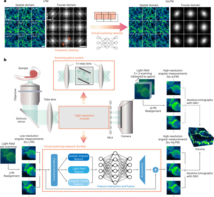
Fig. 1
Principle of VsLFM.
a , Principle of VsLFM using a physics-based deep neural network (Vs-Net) to extract the high-frequency information from the frequency aliasing in traditional LFM induced by diffraction of a small mic...
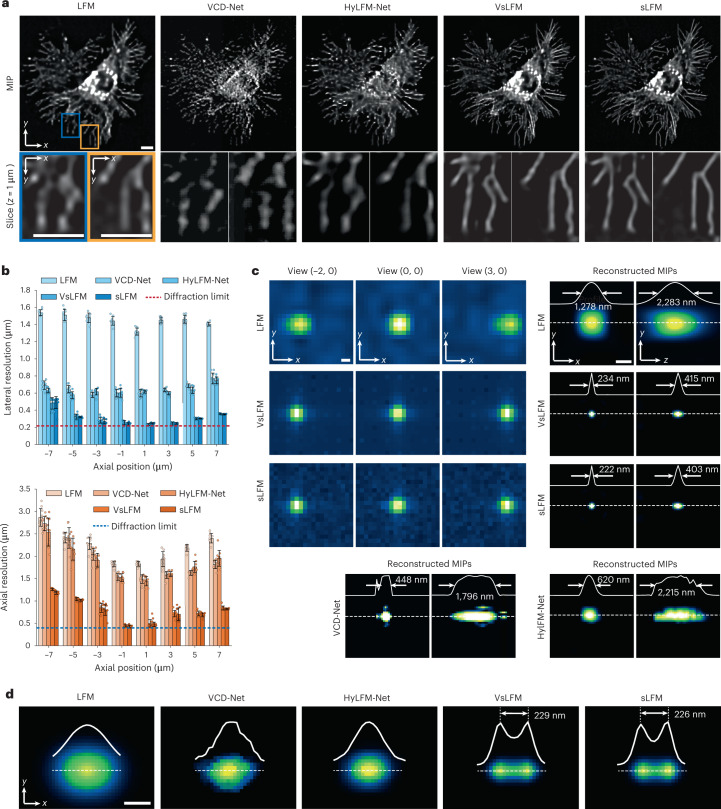
Fig. 2
Resolution enhancement of VsLFM.
a , MIPs and enlarged regions from xy slices at z =u20091u2009u03bcm of a fixed L929 cell with membrane labeling (TSPAN4-mCherry), obtained by LFM, VCD-Net, HyLFM-Net, VsLFM and sLFM, respectively. b ...
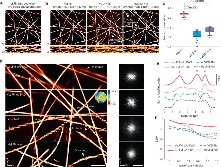
Fig. 3
VsLFM shows robustness to noise and optical aberrations.
a , Orthogonal MIPs of 1-u03bcm-diameter synthetic tubulins, acquired by sLFM with a u00d763/1.4u2009NA oil-immersion objective in ideal imaging conditions, regarded as ground truth. b , VsLFM, VCD-Ne...
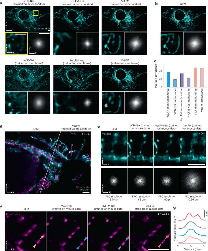
Fig. 4
VsLFM has better generalization ability than end-to-end networks.
a , MIPs and enlarged views of a fixed L929 cell with mitochondria labeling (TOM20-GFP), obtained by VCD-Net, HyLFM-Net and VsLFM trained on the same type of sample (mitochondria, upper row) and a dif...
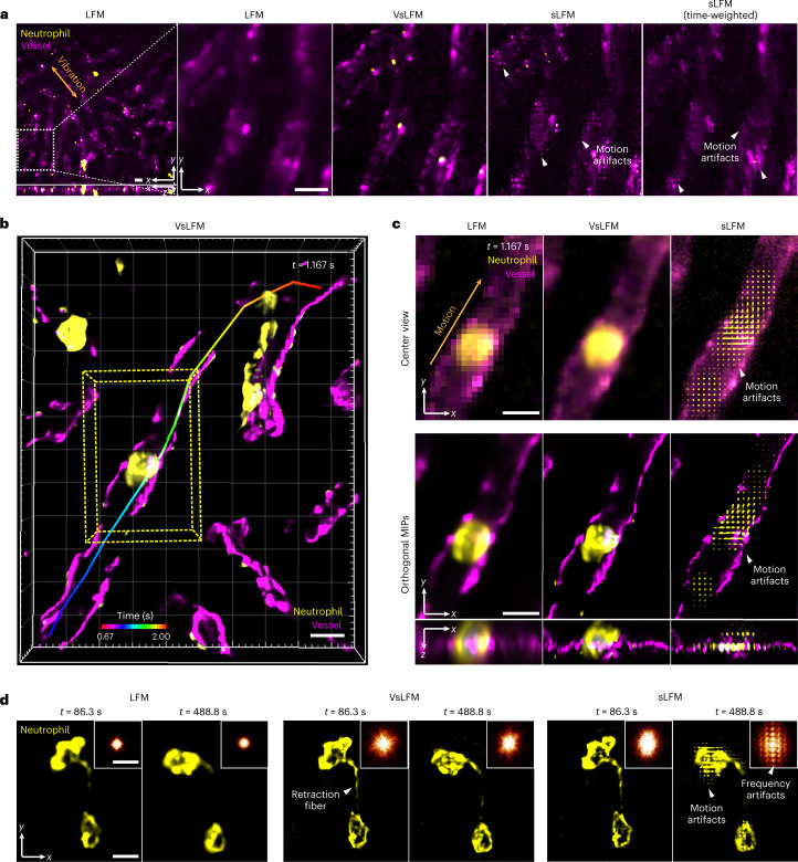
Fig. 5
Long-term high-speed imaging of subcellular dynamics in living mouse livers.
a , Whole-FOV and enlarged MIPs of neutrophils and vessels in a living mouse liver with strong motions induced by respiration, obtained by LFM, VsLFM, sLFM and sLFM with the time-weighted algorithm, r...
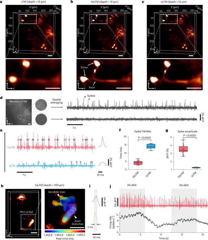
Fig. 6
In vivo high-resolution volumetric voltage imaging of sparsely labeled neurons in Drosophila at 500u2009vps.
a u2013 c , 3D rendering volumes and enlarged MIPs of PPL1 dopamine neurons at a depth of 15u2009u03bcm in Drosophila brain ( MB065B-GAL4 > 20u00d7UAS-pAce ), obtained by LFM ( a ), VsLFM ( b ) and sL...
Figure images are served from the NIH/NLM PubMed Central Open Access Subset or Europe PMC; copyright remains with the publishers and authors.
💬 Discussion
0 commentsNo comments yet. Be the first to start a discussion!
Leave a Comment