Abstract
Clathrin-mediated endocytosis is an essential process that forms vesicles from the plasma membrane. Although most of the protein components of the endocytic protein machinery have been thoroughly characterized, their organization at the endocytic site is poorly understood. We developed a fluorescence microscopy method to track the average positions of yeast endocytic proteins in relation to each other with a time precision below 1 s and with a spatial precision of ~10 nm. With these data, integrated with shapes of endocytic membrane intermediates and with superresolution imaging, we could visualize the dynamic architecture of the endocytic machinery. We showed how different coat proteins are distributed within the coat structure and how the assembly dynamics of N-BAR proteins relate to membrane shape changes. Moreover, we found that the region of actin polymerization is located at the base of the endocytic invagination, with the growing ends of filaments pointing toward the plasma membrane.
🔬 Techniques
🧬 Organisms
💻 Software
✨ Fluorophores
🧪 Sample Preparation
🏭 Microscope Brands
🧪 Reagent Suppliers
📷 Detectors
🎨 Filters
💻 Software Details
📋 Protocols
💾 Data Repositories
🏛️ Research Organizations (ROR)
Affiliated research institutions:
📋 Methods
Strains and plasmids
Yeast strains ( Table 2 ) were generated by homologous recombination of the target genes with PCR cassettes. C-terminal tagging was performed using plasmids pFA6a-EGFP-His3MX6, pFA6a-mCherry-KanMX4 and pYM12-PKS134 for monomeric GFP (myEGFP). pMaM17 ( Khmelinskii et al., 2012 ) was used for the tandem tag of mCherry and sfGFP. pMK03-SNAP-His3MX6 was generated by replacing EGFP with SNAPf ( Sun et al., 2011 ) in pFA6a-EGFP-His3MX6. N-terminal tagging was performed using plasmid pMaM173 which was transformed into yeast strains with a Gal L - ISCE1 integration used to loop out the URA marker and the TEF promoter ( Khmelinskii et al., 2011 ). pMaM175 was used to tag Nuf2 C-terminally with sfGFP ( Khmelinskii et al., 2011 ). The strains used for protein abundance measurements were confirmed by sequencing of the integrated tags. 10.7554/eLife.04535.022 Table 2.
Yeast strains
DOI: http://dx.doi.org/10.7554/eLife.04535.022 Strain # Genotype MKY0216 MATa, his3-∆200, leu2-3,112, ura3-52, lys2-801, NUF2-EGFP::HIS3MX6 MKY0217 MATα, his3-∆200, leu2-3,112, ura3-52, lys2-801, NUF2-EGFP::HIS3MX6 MKY0711 MATa, his3-∆200, leu2-3,112, ura3-52, lys2-801, MYO5-EGFP::HIS3MX6, ABP1-mCherry::kanMX4 MKY0822 MATa, his3-∆200, leu2-3,112, ura3-52, lys2-801, SLA1-EGFP::HIS3MX6, ABP1-mCherry::kanMX MKY1304 MATa, his3-∆200, leu2-3,112, ura3-52, lys2-801, END3-EGFP::HIS3MX6, ABP1-mCherry::kanMX4 MKY1318 MATa, his3-∆200, leu2-3,112, ura3-52, lys2-801, RVS167-EGFP::HIS3MX6, ABP1-mCherry::kanMX4 MKY1368 MATα, his3-∆200, leu2-3,112, ura3-52, lys2-801, LAS17-EGFP::HIS3MX6, ABP1-mCherry::kanMX4 MKY2119 MATα, his3-∆200, leu2-3,112∆::GalL-ISce1-natNT2, ura3-52, lys2-801, sfGFP-SLA2-mCherry::hphNT1 MKY2653 MATa, his3-∆200, leu2-3,112, ura3-52, lys2-801 with pMK0100[CEN, URA3 GFP-ACT1] MKY2655 MATa, his3-∆200, leu2-3,112, ura3-52, lys2-801, ABP1-mCherry::kanMX4 with pMK0100[CEN, URA3 GFP-ACT1] MKY2689 MATα , his3-∆200, leu2-3,112∆::GalL-ISce1-natNT2, ura3-52, lys2-801, sfGFP-SLA2 MKY2720 MATa, his3-∆200, leu2-3,112, ura3-52, lys2-801, ARC18-myEGFP::natNT2, ABP1-mCherry::kanMX MKY2747 MATa, his3-∆200, leu2-3,112, ura3-52, lys2-801, ARC18-myEGFP::natNT2 MKY2832 MATa , his3-∆200, leu2-3,112, ura3-52, lys2-801, RVS167-EGFP::HIS3MX6 MKY2833 MATa, his3-∆200, leu2-3,112, ura3-52, lys2-801, SLA1-EGFP::HIS 3MX6 MKY2834 MATα, his3-∆200, leu2-3,112, ura3-52, lys2-801, ABP1-EGFP::HIS3MX6 MKY2836 MATα, his3-∆200, leu2-3,112∆::GalL-ISce1-natNT2, ura3-52, lys2-801, sfGFP-SLA2, ABP1-mCherry::kanMX MKY3135 MATα, his3-∆200, leu2-3,112∆::GalL-ISce1-natNT2, ura3-52, lys2-801, sfGFP-SLA2, ABP1-mCherry::kanMX, Sla1-SNAP::HIS3MX6 MKY2859 MATa, his3-∆200, leu2-3,112, ura3-52, lys2-801, SLA2-EGFP::HIS3MX6 MKY2863 MATa, his3-∆200, leu2-3,112, ura3-52, lys2-801, CSE4-EGFP::HIS3MX6 MKY2864 MATa, his3-∆200, leu2-3,112, ura3-52, lys2-801, LAS17-EGFP::HIS3MX6 MKY2876 MATa, his3-∆200, leu2-3,112, ura3-52, lys2-801, MYO5-EGFP::HIS3MX6 MKY2880 MATa, his3-∆200, leu2-3,112, ura3-52, lys2-801, ABP1-mCherry-sfGFP::kanMX4 MKY2893 MATa, his3-∆200, leu2-3,112, ura3-52, lys2-801, END3-EGFP::HIS3MX6 MKY2918 MATα, his3-∆200, leu2-3,112, ura3-52, lys2-801, SLA2-EGFP::HIS3MX6, ABP1-mCherry::kanMX4 MKY2919 MATa, his3-∆200, leu2-3,112∆::GalL-ISce1-natNT2, ura3-52, lys2-801, NUF2-sfGFP::KIURA3 MKY2920 MATα, his3-∆200, leu2-3,112∆::GalL-ISce1-natNT2, ura3-52, lys2-801, NUF2-sfGFP::KIURA3 MKY3136 MATa, his3-∆1, leu2-∆0, ura3-∆0, met15-∆0, LAS17-myEGFP::natNT2 MKY3137 MATa, his3-∆1, leu2-∆0, ura3-∆0, met15-∆0, RVS167-myEGFP::natNT2 The yeast strains used in this study.
Show full methods section
Strains and plasmids
Yeast strains ( Table 2 ) were generated by homologous recombination of the target genes with PCR cassettes. C-terminal tagging was performed using plasmids pFA6a-EGFP-His3MX6, pFA6a-mCherry-KanMX4 and pYM12-PKS134 for monomeric GFP (myEGFP). pMaM17 ( Khmelinskii et al., 2012 ) was used for the tandem tag of mCherry and sfGFP. pMK03-SNAP-His3MX6 was generated by replacing EGFP with SNAPf ( Sun et al., 2011 ) in pFA6a-EGFP-His3MX6. N-terminal tagging was performed using plasmid pMaM173 which was transformed into yeast strains with a Gal L - ISCE1 integration used to loop out the URA marker and the TEF promoter ( Khmelinskii et al., 2011 ). pMaM175 was used to tag Nuf2 C-terminally with sfGFP ( Khmelinskii et al., 2011 ). The strains used for protein abundance measurements were confirmed by sequencing of the integrated tags. 10.7554/eLife.04535.022 Table 2.
Yeast strains
DOI: http://dx.doi.org/10.7554/eLife.04535.022 Strain # Genotype MKY0216 MATa, his3-∆200, leu2-3,112, ura3-52, lys2-801, NUF2-EGFP::HIS3MX6 MKY0217 MATα, his3-∆200, leu2-3,112, ura3-52, lys2-801, NUF2-EGFP::HIS3MX6 MKY0711 MATa, his3-∆200, leu2-3,112, ura3-52, lys2-801, MYO5-EGFP::HIS3MX6, ABP1-mCherry::kanMX4 MKY0822 MATa, his3-∆200, leu2-3,112, ura3-52, lys2-801, SLA1-EGFP::HIS3MX6, ABP1-mCherry::kanMX MKY1304 MATa, his3-∆200, leu2-3,112, ura3-52, lys2-801, END3-EGFP::HIS3MX6, ABP1-mCherry::kanMX4 MKY1318 MATa, his3-∆200, leu2-3,112, ura3-52, lys2-801, RVS167-EGFP::HIS3MX6, ABP1-mCherry::kanMX4 MKY1368 MATα, his3-∆200, leu2-3,112, ura3-52, lys2-801, LAS17-EGFP::HIS3MX6, ABP1-mCherry::kanMX4 MKY2119 MATα, his3-∆200, leu2-3,112∆::GalL-ISce1-natNT2, ura3-52, lys2-801, sfGFP-SLA2-mCherry::hphNT1 MKY2653 MATa, his3-∆200, leu2-3,112, ura3-52, lys2-801 with pMK0100[CEN, URA3 GFP-ACT1] MKY2655 MATa, his3-∆200, leu2-3,112, ura3-52, lys2-801, ABP1-mCherry::kanMX4 with pMK0100[CEN, URA3 GFP-ACT1] MKY2689 MATα , his3-∆200, leu2-3,112∆::GalL-ISce1-natNT2, ura3-52, lys2-801, sfGFP-SLA2 MKY2720 MATa, his3-∆200, leu2-3,112, ura3-52, lys2-801, ARC18-myEGFP::natNT2, ABP1-mCherry::kanMX MKY2747 MATa, his3-∆200, leu2-3,112, ura3-52, lys2-801, ARC18-myEGFP::natNT2 MKY2832 MATa , his3-∆200, leu2-3,112, ura3-52, lys2-801, RVS167-EGFP::HIS3MX6 MKY2833 MATa, his3-∆200, leu2-3,112, ura3-52, lys2-801, SLA1-EGFP::HIS 3MX6 MKY2834 MATα, his3-∆200, leu2-3,112, ura3-52, lys2-801, ABP1-EGFP::HIS3MX6 MKY2836 MATα, his3-∆200, leu2-3,112∆::GalL-ISce1-natNT2, ura3-52, lys2-801, sfGFP-SLA2, ABP1-mCherry::kanMX MKY3135 MATα, his3-∆200, leu2-3,112∆::GalL-ISce1-natNT2, ura3-52, lys2-801, sfGFP-SLA2, ABP1-mCherry::kanMX, Sla1-SNAP::HIS3MX6 MKY2859 MATa, his3-∆200, leu2-3,112, ura3-52, lys2-801, SLA2-EGFP::HIS3MX6 MKY2863 MATa, his3-∆200, leu2-3,112, ura3-52, lys2-801, CSE4-EGFP::HIS3MX6 MKY2864 MATa, his3-∆200, leu2-3,112, ura3-52, lys2-801, LAS17-EGFP::HIS3MX6 MKY2876 MATa, his3-∆200, leu2-3,112, ura3-52, lys2-801, MYO5-EGFP::HIS3MX6 MKY2880 MATa, his3-∆200, leu2-3,112, ura3-52, lys2-801, ABP1-mCherry-sfGFP::kanMX4 MKY2893 MATa, his3-∆200, leu2-3,112, ura3-52, lys2-801, END3-EGFP::HIS3MX6 MKY2918 MATα, his3-∆200, leu2-3,112, ura3-52, lys2-801, SLA2-EGFP::HIS3MX6, ABP1-mCherry::kanMX4 MKY2919 MATa, his3-∆200, leu2-3,112∆::GalL-ISce1-natNT2, ura3-52, lys2-801, NUF2-sfGFP::KIURA3 MKY2920 MATα, his3-∆200, leu2-3,112∆::GalL-ISce1-natNT2, ura3-52, lys2-801, NUF2-sfGFP::KIURA3 MKY3136 MATa, his3-∆1, leu2-∆0, ura3-∆0, met15-∆0, LAS17-myEGFP::natNT2 MKY3137 MATa, his3-∆1, leu2-∆0, ura3-∆0, met15-∆0, RVS167-myEGFP::natNT2 The yeast strains used in this study.
Live-cell imaging
Yeast cells were grown to logarithmic phase on SC-Trp medium at 25°C. They were adhered to ConA coated coverslips. Cells were incubated for 10 min at room temperature on the ConA coated coverslip and then washed with SC-Trp medium. Cells were imaged on the coverslip in 40 µl of SC-Trp medium. All samples were imaged at room temperature using an Olympus IX81 wide-field epifluorescence microscope equipped with a 100×/1.45 objective. For single channel live cell imaging 488 nm laser light and images were acquired with 80–100 ms exposure time. Emission light was filtered using the GFP-3035C-OMF single-band filter set (Semrock, Rochester, NY). Fluorescence was detected using the Hamamatsu ImagEM EMCCD camera. For two color live cell imaging the samples were excited simultaneously with 488 nm and 561 nm laser light for 250 ms exposure. Excitation light was reflected with a OBS-U-M2TIR 488/561 (Semrock, Rochester, NY) dichroic mirror. Emission light was split and filtered with the DUAL-view (Optical Insights, LLC, Tucson, AZ) beam splitter. The beam splitter created two separated images, one for each channel, on the Hamamatsu ImagEM EMCCD camera sensor. Photobleaching was performed using a custom built setup with a 488 nm laser, focused on a ∼0.5 µm spot. The wide-field epifluorescence microscope setup was controlled by Metamorph 7.5 (Molecular Devices, Sunnyvale, CA).
Image analysis
Before tracking the endocytic patches and the photobleaching experiments, the extracellular background was subtracted from the images using the Background Subtraction function in ImageJ (with rolling ball radius equal to 90 pixels, corresponding to 9 µm). To correct for photobleaching, each image was then scaled such that the average fluorescence intensity within the cell remains constant in successive frames. To correct for the uneven cytoplasmic background signal at the edge of the cell, we estimated the cytoplasmic contribution by further processing the images with a median filter (of kernel 6 pixels, corresponding to 0.6 µm). We then subtracted the cytoplasmic background and tracked endocytic patches using the Particle Tracker plugin in ( Sbalzarini and Koumoutsakos, 2005 ).
Single channel trajectory alignment and averaging
Each protein trajectory p is a list of points, p i = { p i x , p i y , p i f } , defined from p i x and p i y , the centroid 2D coordinates in the focal plane, and p i f , the corresponding fluorescence intensity, where the index i denotes time. Trajectories were aligned in space and time by a custom made software written in R ( www.CRAN.org ). An isometric transformation of space T = { T x , T y , T θ } is defined as T : { x , y } → { cos ( T θ ) x − sin ( T θ ) y + T x , sin ( T θ ) x + cos ( T θ ) y + T y } . The best alignment between two trajectories, p and q , is computed by minimizing the sum of the squared difference between all overlapping points: { T b e s t , τ b e s t } = arg min T , τ ( ∑ i w i ( ( q i + τ x − ( T p i ) x ) 2 + ( q i + τ y − ( T p i ) y ) 2 ) ∑ i w i ) , with w i = q i + τ f p i f . In practice, we computed for each possible time shift τ , the best spatial transformation ( Horn, 1987 ), and selected the best overall result. The weights w i are the product of the fluorescence intensities of the spot pairs at each time point. Being proportional to the cross-correlation in time of the fluorescence intensities, they helped to refine the temporal alignment of the trajectories. To not bias the alignment by the choice of a reference, each trajectory was separately used as a reference to which all the remaining trajectories were aligned. Given n trajectories we thus computed n(n−1) alignments. Each alignment gave us an estimate of the transformation that aligns a trajectory to its reference. We thus estimated the average transformation that aligns all the trajectories together as seen from a common reference point in the field of view. Once aligned, all trajectories were averaged to obtain the average trajectory. The average trajectory of each protein was derived from 50 to 80 individual trajectories ( Figure 1—figure supplement 1 , Table 1 ). See Source code 1. The alignment of the trajectories of Abp1, Arc18 and Act1 was computed using only the trajectory data associated with the invagination dynamics, up to the trajectory peak in fluorescence intensity. The number of molecules over time was obtained after calibrating the fluorescence intensity curve mean integral with the average number of molecules estimated at the endocytic spot (see ‘Materials and Methods’: calibration of the fluorescence intensity curve of the trajectories with the number of molecules). All data presented in this work are listed in the Supplementary file 1 . All the curves in Figure 7 , except Las17 and Myo5, were smoothened using a Savitzky-Golay filter over 11 time points. Las17 and Myo5 were smoothened using a moving average filter of length 5. Two color alignment procedure The alignment is performed using pairs of trajectories acquired simultaneously with two labeled proteins: Abp1-mCherry serving as a reference, and a protein of interest tagged with GFP. Simultaneous acquisition of the two colors is made with the DUAL-view beam splitter (Optical Insights, LLC, Tucson, AZ). Image un-splitting and correction of chromatic aberration are done following the DUAL-view recommended procedures. A sample with TetraSpeck microsphere (0.1 µm, Invitrogen, Carlsbad, CA) was imaged in both channels and the centroids were identified with Particle Tracker ( Sbalzarini and Koumoutsakos, 2005 ) in ImageJ and then processed in MATLAB (TheMathworks, Natick, MA) to generate a spatial warping transformation that was applied on the raw coordinates. The non-linear transformation was generated by the local weighted mean (lwm) method of cp2tform (See Matlab help and references thereafter). Definitions The average trajectory of a protein, P , is represented by a temporal collection of 6-dimensional vectors, P i = { P i x , P i y , P i f , δ i x , δ i y , δ i f } with i = { 1 , … , N } . P contains P x and P y , the average position of the centroid of the fluorescence patch, and the corresponding average fluorescence P f , the standard error of the means δ x and δ y , associated with the position coordinates, and δ f , the standard error of the mean associated with the fluorescence intensity. The average trajectory of the reference protein, that we name R , follows the same notation. The trajectory pairs are not necessarily defined over the same time interval as the average trajectories P and R . They were thus smoothed with a moving average, to reduce noise, and interpolated with a cubic spline to estimate values at the missing time points. The resulting trajectory, p is a temporal collection of 3-dimensional vectors p i = { p i x , p i y , p i f } with i = { 1 , … , N } , built from the positions, p x and p y , and the fluorescence intensities p f of each endocytic patch. The notation is similar for the reference trajectory r . r and p are already aligned together because they were acquired simultaneously.
Temporal alignment
First, individual trajectories are aligned to their corresponding average trajectory in time. The resulting lag τ p , that aligns in time p and P , is the one that maximizes the cross-correlation of the fluorescence intensities: τ p = arg max τ ( ∑ i p i + τ f P i f ) . The same procedure is used to compute the lag τ r between r and R .
Spatial alignment
An isomeric transformation of space T = { T x , T y , T θ } is the combination of a translation and a rotation T : { x , y } → { cos ( T θ ) x − sin ( T θ ) y + T x , sin ( T θ ) x + cos ( T θ ) y + T y } . The optimal transformation Tp that aligns p to P is calculated as T p = arg min T ( ∑ i w i ( ( P i x − ( T p i + τ p ) x ) 2 + ( P i y − ( T p i + τ p ) y ) 2 ) ∑ i w i ) , with w i = P i f p i + τ p f δ i x δ i y . The same procedure is used to compute T r that aligns r to R . The spatial alignment of the trajectories of Abp1, Arc18 and Act1 was computed using only the trajectory data associated with the invagination dynamics, up to the trajectory peak in fluorescence intensity. Estimate of the average transformations Between 50 and 350 trajectory pairs were used to compute the average alignment ( Table 1 ). For each trajectory pair, we got an estimate of the transformations that align r to R and p to P . An estimate of the transformation that aligns P to R is thus the combination of the inverse transformation that aligns p to P and of the transformation that aligns r to R : T = T r ( T p ) − 1 . The average transformation is then the average of the estimates of the individual transformations that align P to R , computed from each of the trajectory pairs. The average time alignment τ is computed as: τ = median ( τ r − τ p ) and δτ is the estimate of the standard error for the median computed as: δ τ = 1.4826 × M A D τ M MAD τ is the median absolute deviation for τ and M is the number of trajectory paires used to compute the average transformation. T x and T y are computed as: T x = median ( T r x − cos ( T r θ − T p θ ) T p x + sin ( T r θ − T p θ ) T p y ) , T y = median ( T r y − sin ( T r θ − T p θ ) T p x − cos ( T r θ − T p θ ) T p y ) . T θ is computed as: T θ = median ( T r θ − T p θ ) . δT x , δT y and δ T θ are computed as δτ using their respective MAD. Note that the approximation used to estimate T θ is only valid if T r θ ≈ T p θ . To ensure that this is the case, R and P are first aligned to their axis of symmetry, which is the direction of the invagination that we defined as the X-axis. As r and p are already aligned along the axis of invagination, because they were acquired simultaneously, the final rotation that align P to R is close to the identity ( T θ ≈ 0 ). Centering P to its center of mass further minimize any error that might be induced by the above approximation. The trajectory of the protein of interest aligned to the reference trajectory is thus: P i ′ = { ( T P i ) x , ( T P i ) y , P i f , ζ i x , ζ i y , ζ i f } , where ζ i x and ζ i y are the standard errors computed as: ζ i x = ( δ i x ) 2 + ( P i y δ T θ ) 2 + ( δ T x ) 2 , ζ i y = ( δ i y ) 2 + ( P i x δ T θ ) 2 + ( δ T y ) 2 . All plots describing the trajectories inward movement along the invagination direction report the 95% confidence intervals, computed as 1.96 × ζ i x and 1.96 × δτ . See Source code 2. Two color averaging procedure used for non-motile proteins Trajectory pairs of Myo5-GFP or Las17-GFP and Abp1-mCherry were used to generate Myo5 and Las17 average trajectories. The rotations and translations that aligned the Abp1-mCherry trajectories and Abp1-GFP average trajectory together were used to align the corresponding Myo5-GFP or Las17-GFP trajectories. Once aligned, the coordinates of the GFP trajectories were averaged together at each time point.
Simulation of the accuracy of the two color alignment procedure
To control the accuracy of our alignment procedure we generated virtual trajectory pairs using two trajectories that we generated as a template (ground truth trajectories): one ground truth trajectory represents the reference protein while the other represents the target protein. The points of the trajectory pairs were randomly generated and were normally distributed around the ground truth trajectories with sigma σ p for the trajectories of the target protein and σ r for the trajectories of the reference protein. All trajectories were generated with the same sampling rate as the real trajectories. The virtual trajectory pairs were then processed with the same pipeline we used for the real data to align the ground truth trajectories together. As the ground truth trajectories were already aligned all transformations are expected to be 0 ( Figure 1—figure supplement 4A–D ). When we arbitrarily increased the noise used to generate both the reference and the target proteins we observed that the alignment procedure remains faithful up to ∼25 nm of noise. For higher values a small systematic shift occurs ( Figure 1—figure supplement 4C ). We then tested the robustness of the alignment procedure keeping σ r fixed at 19 nm while we varied σ p . A σ r fixed mimics the noise in the real trajectory pairs, as the reference protein was always imaged under the same conditions. The alignment showed negligible errors ( Figure 1—figure supplement 3E–L ). Note that in the real trajectory pairs σ p span a range from 10 nm to 24 nm, however the algorithm was stable also for higher errors. We observed a systematic shift, of maximally ∼3 nm, that occurs when the trajectories are getting far from the reference ( Figure 1—figure supplement 3K ). This is expected as any small error in the alignment of the trajectories leads to an underestimate of the separation between the reference and the target protein. This underestimate grows larger the bigger the separation is, resulting in the trajectory of the target protein being shifted little closer to its reference than it should be. A shift of 3 nm is reached when the trajectories are 30 nm away far from the reference protein, which is the maximal distance of a trajectory from its reference in our model. Simulation of the robustness to systematic shifts between the two channels during two color acquisition To test for the robustness against systematic shifts between the two channels, we shifted the reference trajectories in the virtual trajectory pairs that we generated on the computer (see ‘Materials and Methods’: Simulation of the accuracy of the two color alignment procedure; σ r = 16 nm and σ r = 19 nm), by shifts up to 150 nm along one direction. These shifts simulate different amounts of aberration between the two channels. On average, the alignment is not affected ( Figure 1—figure supplement 4A ). In fact, the trajectory pairs, as well as the endocytic events that they mimic, are oriented in all possible directions and once their average relative position is calculated, the chromatic aberration contribution is averaged out. However, the incertitude in the average position increases, as expected ( Figure 1—figure supplement 4A ). It is important to note that our pixel size correspond to 100 nm, therefore any shift larger than 50–100 nm would have been easily noticeable by eye. To assess how the alignment of the real data would be affected by a systematic color shift we also shifted the real trajectory pairs we used to align Sla2-GFP tp Abp1-GFP. Again, we induced shifts up to 150 nm to the trajectories of Abp1-mCherry to simulate different amounts of aberration between the two channels. The average position of Sla2-GFP does not significantly change but the incertitude in its average position increases ( Figure 1—figure supplement 4B–D ).
Simulation of the accuracy of the trajectory averaging
To test the accuracy of the trajectory averaging we generated 65 virtual trajectories starting from a trajectory template (ground truth trajectory). The trajectories were generated adding noise that was normally distributed around the points of the ground truth trajectory with a standard deviation σ . We sampled values of σ covering the range of noise encountered experimentally (between 10 nm and 20 nm). The average trajectories where then aligned in time and in space to a reference trajectory that was generated together with the ground truth trajectory. To compute the alignment we used virtual trajectory pairs generated from the ground truth trajectory and the reference trajectory as described in ‘Materials and Methods: simulation of the accuracy of the two color alignment procedure’, with noises σ p = 10 nm and σ r = 19 nm respectively. The averaging procedure and the complete alignment procedure are very robust: after the alignment the average trajectories were reproducing very closely the ground truth trajectory ( Figure 1—figure supplement 5 ). As expected, the average of very noisy trajectories slightly underestimates the full length of the ground truth trajectory ( Figure 1—figure supplement 5D ).
Quantification of the number of molecules
To quantify the protein amounts we imaged a sample containing cells from both a yeast strain expressing a fluorescently tagged protein of interest and a yeast strain expressing fluorescently tagged Nuf2, which was used as a reference to calibrate the fluorescence intensity ( Joglekar et al., 2006 ). Both strains expressed the same fluorescent tag and were imaged together. For the quantification of the Nuf2 fluorescence intensity we used cells in anaphase-telophase only. Excitation light and emission light were directed through the U-MGFPHQ (Olympus, Japan). Samples were imaged as a z-stack of 21 frames, 200 nm spaced, using the Hamamatsu Orca-ER CCD camera. Each frame was excited with X-Cite 120Q lamp for 400 ms. Frames were not processed for background subtraction and the spots were quantified by quantifying the fluorescence intensity of the patches, in the frame of the z-stack in which they were brighter, and subtracting their local background, as described in Joglekar et al. (2006) . The intensities of the fluorescent patches of the target endocytic proteins where in general dimmer than Nuf2, and their distribution was in general not symmetric. The intensities measured from the patches of the target proteins were thus processed after a logarithmic transformation. The average number of molecules of the target protein n p was derived as: n p = f g n r . n r is the known number of molecules of the reference, f is the median of the fluorescence intensity of the patches of the target protein and g is the median fluorescence intensity of the patches of the reference protein. The uncertainty in the number of molecules was derived as: (1) δ n p = ( n r f g δ l ) 2 + ( n r f g 2 δ g ) 2 + ( f g δ n r ) 2 . δ l is the estimate of the standard error for the median of the fluorescence intensity of the target protein after logarithmic transformation, l = log( f ), and is computed as: δ l = 1.4826 × M A D l N . MAD l is the median absolute deviation for l and N is the number of observations. The distribution of the intensities of the target endocytic proteins where not symmetric, they were thus processed after a logarithmic transformation of their intensities. δ g is computed as δ l , using MAD g , the median absolute deviation of the fluorescence intensity of the reference protein. δn r is the uncertainty in Nuf2 number of molecules. The average number of molecules n p was then used to rescale fluoresce intensity curves of the average trajectories (see ‘Materials and Methods’: calibration of the fluorescence intensity curve of the trajectories with the number of molecules). Nuf2 number of molecules was quantified using Cse4 as a reference. The number of Cse4 molecules used for the calibration was 5 molecules/kinetochore ( Lawrimore et al., 2011 ). The measured average number of Nuf2 molecules, per fluorescent spot, was 280.6 ± 16.1 molecules. Its error was quantified as in Eq.(1) with δn r = 0. The quantification of Nuf2 molecules with Cse4 served as a control for our procedure as there is no difference in the ratio between our number of Nuf2 molecules and the number of Cse4 molecules, which is 3.5 ± 0.2 Nuf2 molecules each Cse4, and Joglekar's ratio, which is 3.5. To quantify the protein abundance of Arc18, which was tagged with myEGFP, we compared the fluorescence intensity of myEGFP and EGFP tags and we measured the myEGFP tags to be 68% ± 14% of the fluorescence intensity of an EGFP tag. The uncertainty in Arc18 number of molecules was then computed as: δ n p = ( c f g n r δ l ) 2 + ( c f g 2 δ g ) 2 + ( c f g δ n r ) 2 + ( f g n r δ c ) 2 . c is the estimate of the correction for the fluorescence intensity and δ c is its uncertainty. Calibration of the fluorescence intensity curve of the trajectories with the number of molecules We calibrated the fluorescence intensity curve P f for each average trajectory, P i = { P i x , P i y , P i f , δ i x , δ i y , δ i f } with i = { 1 , … , N } , to estimate of the number of molecules P n over time. P n is computed by rescaling the fluorescence intensity curve of the protein of interest with the average number of molecules n p at the endocytic site (see ‘Materials and methods’: quantification of the number of molecules): P i n = n P P i f − P min f 1 N ∑ j = 1 N ( P j f − P min f ) , with P min f = min k ( P k f ) The error in the estimate of the number of molecules is: δ i n = ( P i f − P min f F ¯ δ n P ) 2 + ( n p N N F ¯ − P i f + P min f F ¯ 2 δ i f ) 2 + ( n p P i f − P min f − F ¯ F ¯ 2 δ m ) 2 , δ m = δ l f with l = arg min j ( P j f ) , F ¯ = 1 N ∑ i = 1 N ( P i f − P min f ) . where δn p is the standard error of the average number of molecules measured in the endocytic fluorescent patches (see ‘Materials and Methods: quantification of the number of molecules). All plots describing the number of molecules report the 95% confidence interval, computed as 1.96 × δ i n .
Quantification of the ratio between GFP-Act1 and the total actin
To quantify the ratio between GFP-Act1 and the total actin we run western blots with cell extract of yeast cells expressing GFP-Act1 (MKY2653) ( Wu and Pollard, 2005 ). MKY2653 cells where grown overnight in SC-URA media. As primary antibody against actin we used Sigma A2066. The secondary antibody was a AP-1000 Alkaline Phosphatase anti-rabbit igG (H + L) from Vector Laboratories. The quantification was repeated 8 times. The ratio r ˜ between GFP-Act1 and the total actin was computed as: r ˜ = r r + 1 where r is the average ratio between the GFP-Act1 and the endogenous actin that we measured from the 8 quantifications. The error was computed as: σ r ˜ = σ r ( r + 1 ) 2 where σ r is the standard error of the mean of r . The direction of Abp1 trajectories with respect to the membrane To determine the angle between Abp1 trajectories and the yeast cell surface, we determined the closest membrane tangent for each Abp1 track, using a binary mask of the yeast cell in which the trajectory was acquired. We then measured the angle between the vector tangent to the membrane and the vector whose direction was determined by the interpolation of Abp1 trajectory points on the focal plane ( Figure 1—figure supplement 2B ). Alignment of photobleaching trajectories Individual photobleaching experiments were tracked with the Particle Tracker ( Sbalzarini and Koumoutsakos, 2005 ) plugin in ImageJ after background subtraction, normalization and cytoplasmatic background subtraction of the images (see ‘Materials and methods’: Image analysis). The tangent to the plasma membrane was determined in ImageJ using a binary mask of the cell. A custom written software in R was then used to extrapolate the trajectory along the direction orthogonal to the plasma membrane, which represents the inward movement of the photobleached endocytic spot. The resulting trajectories were aligned in time and in space to the average trajectory of the corresponding protein using the fluorescence intensity curve and the inward movement of the average trajectory and of the photobleached trajectory before the photobleaching. After alignment, the photobleached trajectories were thus aligned in space and time with all the average trajectories and with the plasma membrane profiles ( Figure 6C–F ). Measuring the displacement of N- and C-termini of Sla2 To check whether Sla2 was oriented on average perpendicularly to the plasma membrane, we tagged simultaneously the N-terminus with sfGFP and the C-terminus with mCherry (GFP-Sla2-RFP, Figure 3—figure supplement 1A ). In cells treated with 2 µM LatA, we recorded the closest membrane tangent to each GFP spot. We then measured the angle between the vector tangent to the membrane and the vector whose direction was determined by the centroids of the corresponding GFP and mCherry spots, for each GFP and mCherry pairs ( Figure 3—figure supplement 1B ). In order to determine whether the displacement between the N- and C-terminal trajectories of Sla2 is a measure for Sla2 length we measured the distance between the N- and C-terminus of Sla2, by tagging simultaneously the N- terminus with GFP and the C-terminus with mCherry ( Figure 3—figure supplement 1A ). We arrested the membrane invagination by treating cells with 2 µM of LatrunculinA (LatA) ( Kukulski et al., 2012 ) and we imaged cells on the GFP and mCherry channels. Images were corrected for chromatic aberration as for the two color trajectories (see ‘Materials and methods’: Two color alignment procedure). The separations between the centroids of the GFP and mCherry pairs follow a non-gaussian distribution ( Stirling Churchman et al., 2006 ), which was used to compute the distance between the fluorophores and thus estimate the displacement of the N- and C-terminal tags of Sla2 ( Figure 3—figure supplement 1C ). The distance is reported in the text together with the estimate of the standard error of the mean obtained from the observed Fisher information matrix. As a control, we performed the same analysis on a TetraSpeck sample ( Figure 3—figure supplement 1D ) and on Sla2 tandemly tagged at its C-terminus with both mCherry and sfGFP ( Figure 3—figure supplement 1E,F ).
Estimation of the membrane area covered by Rvs
To estimate the membrane area covered by the Rvs161/167 proteins, we assumed that all protein molecules are membrane bound and homogeneously distributed on the surface of the endocytic invagination. Their distribution was computed considering that BAR proteins form a dimer that is ∼13 nm long ( Peter et al., 2004 ) and tubulate in vitro forming spirals spaced by 50 Å ( Mim et al., 2012 ). We used those data, together with our estimate of the number of Rvs molecules and with the average membrane shapes, to model all possible coverages of the invagination along the invagination length. We then chose the coverage whose center of mass matched the position of the Rvs167-GFP average trajectory. We extrapolated the plasma membrane profiles to estimate the plasma membrane shape at time 0 in order to determine the Rvs coverage just prior to scission. Estimation of Abp1 patch lifetime ( Figure 1—figure supplement 2A ) Abp1 lifetimes were estimated from the lifetime of the trajectories (i.e. the time difference between the first and the last time point in the trajectory). We considered only the trajectories that were complete and, to minimize as much as possible the effect of photobleaching, we considered only the trajectories that were recorded in a number of frames, at the beginning of the video, covering ∼3 times the known lifetime of the protein. Note that to achieve robust automatic patch detection the thresholding of the fluorescent patches was stringent, resulting in Abp1 patch lifetimes that are an underestimate of the true patch lifetime.
Sample preparation for superresolution microscopy
ConA crosslinked glass coverslips were prepared as described previously ( Mund et al., 2014 ). 24 mm coverslips were cleaned for at least 12 hr in 1:1 methanol/hydrochloric acid, and washed in ddH 2 O until the pH of the solution remained neutral. 20 µl of Bioconext (UCT, Bristol, PA) was spread out over the coverslip and incubated for 30 min, followed by washing twice with ethanol, twice with H 2 O, drying at 65°C for 30 min and incubation for 60 min with 20 µl of 2% ConA. Coverslips were then rinsed three times with H 2 O, air dried and stored until usage. Sample preparation was performed as described previously ( Mund et al., 2014 ). In summary, yeast cells were grown in SC-Trp medium until reaching log phase, pelleted by centrifugation, resuspended in a small volume of ddH 2 O and pipetted on the ConA crosslinked glass coverslips. After settling for 15 min, the supernatant was removed and the coverslips were submerged in a fixative containing 4% formaldehyde, 2% sucrose in PBS for 15 min. Cells were then incubated two times for 15 min in PBS containing 50 mM NH 4 Cl to stop the fixation. Coverslips were subsequently put face down on a 100 μl drop of blocking solution consisting of 50% ImageIT FX (Invitrogen, Carlsbad, CA) to block background due to unspecific binding and 0.25% Triton-100 in PBS for 60. Coverslips were briefly washed three times with PBS and put face down on a 100 µl drop of SNAP labeling solution containing 1 µM SNAP-Surface Alexa Fluor 647, 1% BSA, 0.25% Triton X-100, 0.004% NaN 3 in PBS and incubated for 120 min. Finally, coverslips were washed three times by gentle shaking in PBS for at least 5 min.
Superresolution microscopy
Localization microscopy was performed on a custom-built microscope. Single-mode output from an iChrome MLE-L laser box equipped with 405 nm, 488 nm, 561 nm and 640 nm laser lines (Toptica Photonics, Germany) was focused onto the back–focal plane of a 60× NA 1.49 TIRF objective (Nikon, Japan) and adjusted for epi illumination. Emission light was filtered using an ET 700/100 bandpass filter (Chroma, Bellows Falls, VT) and a FF01-446/523/600/677 multi bandpass filter (Semrock, Rochester, NY), and focused by a 400 mm tube lens onto the chip of an EMCCD camera (Ixon Ultra, Andor, United Kingdom) that was air-cooled to −75°C. Images were acquired using MicroManager ( Edelstein et al., 2010 ). A piezo objective positioner (Physikinstrumente, Karlsruhe, Germany) was used to move the z-focus. The focus was stabilized by an electronic feedback loop based on an infrared laser that was totally internally reflected at the coverslip and detected by a quadrant photodiode. The z stability was better than ±10 nm over several hours. Lateral drift, typically smaller than 50 nm/hr, was corrected for in the analysis software. Image acquisition was performed as described ( Mund et al., 2014 ). In brief, the samples were mounted in a custom-made holder and covered with at least 200 µl of imaging buffer consisting of 150 mM Tris–HCl pH7.5, 2% glucose, 60 mM cysteamine, 40 µg/ml catalase and 0.5 mg/ml glucose oxidase. We used an exposure time of 25 ms and an EM gain of 100. Imaging laser intensity at 640 nm was 2.5 kW/cm 2 , the activation laser intensity was automatically adjusted to ensure a constant number of localizations per frame. Typically 30,000–50,000 frames were recorded. Localization analysis was performed as previously described ( Ries et al., 2012 ). In summary, photon counts were obtained by subtraction of the constant offset from the pixel count and multiplication with the inverse gain. Initially, approximate positions of bright spots were determined by smoothing, nonmaximum suppression and thresholding. Selected peaks were fitted by a pixelized Gaussian function and a homogenous photonic background with a maximum likelihood estimator for Poisson distributed data using a freely available, GPU based fitting routine (Smith et al., 2010) on a Geforce GTX670 (Nvidia, Santa Clara, CA). Lateral drift correction was performed using image correlation as previously described. Localizations with an uncertainty of >15 nm were discarded. The images in Figure 3 and Figure 3—figure supplement 2 were rendered using a Gaussian with a width according to the respective localization precision. All analysis software was written in Matlab (TheMathworks, Natick, MA). The observed structures in Figure 3—figure supplement 2 were visually classified. ‘Clear ring structures’ show both localizations in circular arrangement and a pore zone in the middle with virtually no localizations, while for ‘Possible ring structures’ one of the two criteria was less striking. ‘No ring structures’ exhibit other geometries.
Two color alignment procedure The alignment is performed using pairs of trajectories acquired simultaneously with two labeled proteins: Abp1-mCherry serving as a reference, and a protein of interest tagged with GFP. Simultaneous acquisition of the two colors is made with the DUAL-view beam splitter (Optical Insights, LLC, Tucson, AZ). Image un-splitting and correction of chromatic aberration are done following the DUAL-view recommended procedures. A sample with TetraSpeck microsphere (0.1 µm, Invitrogen, Carlsbad, CA) was imaged in both channels and the centroids were identified with Particle Tracker ( Sbalzarini and Koumoutsakos, 2005 ) in ImageJ and then processed in MATLAB (TheMathworks, Natick, MA) to generate a spatial warping transformation that was applied on the raw coordinates. The non-linear transformation was generated by the local weighted mean (lwm) method of cp2tform (See Matlab help and references thereafter).
Two color averaging procedure used for non-motile proteins Trajectory pairs of Myo5-GFP or Las17-GFP and Abp1-mCherry were used to generate Myo5 and Las17 average trajectories. The rotations and translations that aligned the Abp1-mCherry trajectories and Abp1-GFP average trajectory together were used to align the corresponding Myo5-GFP or Las17-GFP trajectories. Once aligned, the coordinates of the GFP trajectories were averaged together at each time point.
Simulation of the accuracy of the two color alignment procedure
To control the accuracy of our alignment procedure we generated virtual trajectory pairs using two trajectories that we generated as a template (ground truth trajectories): one ground truth trajectory represents the reference protein while the other represents the target protein. The points of the trajectory pairs were randomly generated and were normally distributed around the ground truth trajectories with sigma σ p for the trajectories of the target protein and σ r for the trajectories of the reference protein. All trajectories were generated with the same sampling rate as the real trajectories. The virtual trajectory pairs were then processed with the same pipeline we used for the real data to align the ground truth trajectories together. As the ground truth trajectories were already aligned all transformations are expected to be 0 ( Figure 1—figure supplement 4A–D ). When we arbitrarily increased the noise used to generate both the reference and the target proteins we observed that the alignment procedure remains faithful up to ∼25 nm of noise. For higher values a small systematic shift occurs ( Figure 1—figure supplement 4C ). We then tested the robustness of the alignment procedure keeping σ r fixed at 19 nm while we varied σ p . A σ r fixed mimics the noise in the real trajectory pairs, as the reference protein was always imaged under the same conditions. The alignment showed negligible errors ( Figure 1—figure supplement 3E–L ). Note that in the real trajectory pairs σ p span a range from 10 nm to 24 nm, however the algorithm was stable also for higher errors. We observed a systematic shift, of maximally ∼3 nm, that occurs when the trajectories are getting far from the reference ( Figure 1—figure supplement 3K ). This is expected as any small error in the alignment of the trajectories leads to an underestimate of the separation between the reference and the target protein. This underestimate grows larger the bigger the separation is, resulting in the trajectory of the target protein being shifted little closer to its reference than it should be. A shift of 3 nm is reached when the trajectories are 30 nm away far from the reference protein, which is the maximal distance of a trajectory from its reference in our model.
Additional files 10.7554/eLife.04535.023 Supplementary file 1. Average trajectory data. The average trajectories plotted in Figures 1–6 t : time points in seconds (time 0 corresponds to the Rvs167 intensity peak). t.err : 95% confidence interval of the time alignment in seconds. x : centroid position, in respect to the plasma membrane and along the invagination axis (nm). x.err : 95% confidence interval of the centroid position, in respect to the plasma membrane and along the invagination axis (nm). n : estimate of number of molecules. n.err : 95% confidence interval of the number of molecules. DOI: http://dx.doi.org/10.7554/eLife.04535.023 10.7554/eLife.04535.024 Source code 1. Average trajectories V0.1. The collection of R functions used to compute the average trajectories. They require the R library Hmisc. DOI: http://dx.doi.org/10.7554/eLife.04535.024 10.7554/eLife.04535.025 Source code 2. Align trajectories V0.2. The collection of R functions used to align the average trajectories together and to plot them. They require the R library MASS and the function plotCI form the R package gregmisc. DOI: http://dx.doi.org/10.7554/eLife.04535.025
📊 Figures
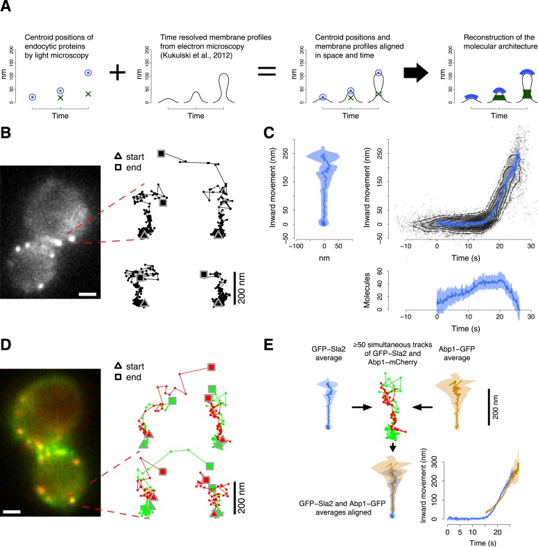
Figure 1.
Tracking procedure.
( A ) The rational behind our approach. The centroid positions of endocytic proteins were correlated with the plasma membrane intermediates derived from CLEM ( Kukulski et al., 2012 ). We could thus p...
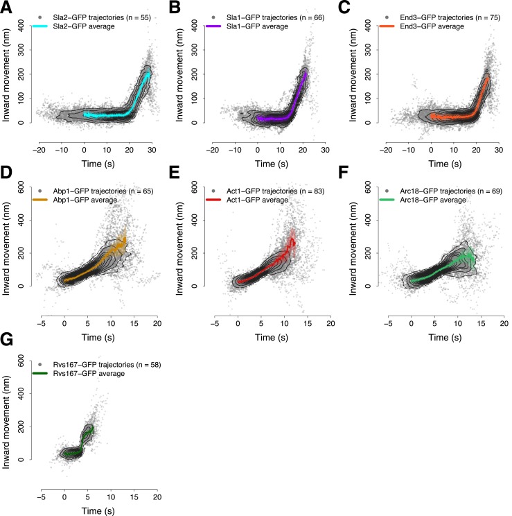
Figure 1u2014figure supplement 1.
Average trajectories of endocytic events.
( A u2013 G ) The average trajectories and the individual trajectories that were used to generate the average trajectories are shown together. The contour lines highlight point densities. The distribu...
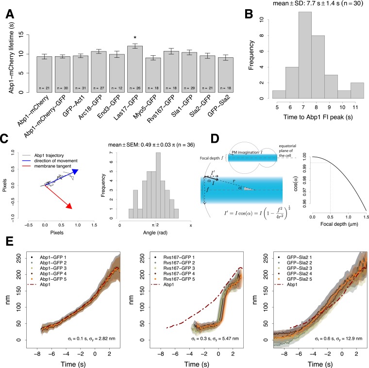
Figure 1u2014figure supplement 2.
Experimental controls for the alignment procedure.
( A ) Lifetimes of Abp1 patches in strains expressing Abp1-mCherry and a target protein labeled with GFP were used to control the functionality of the tagged proteins. Only Las17-GFP strain showed a s...
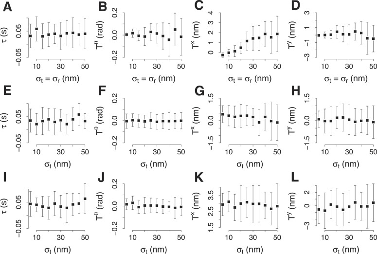
Figure 1u2014figure supplement 3.
Simulation of the accuracy of the two color alignment procedure.
( A u2013 D ) Lag u03c4 , rotation T u03b8 , and translations, T x and T y , that align a virtual trajectory to its virtual reference. The trajectory and its reference were generated already aligned a...
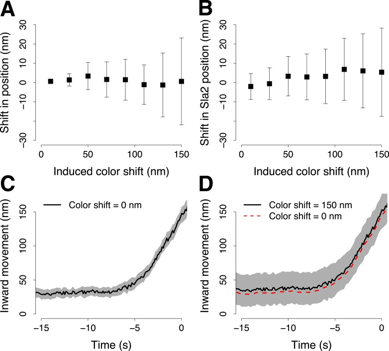
Figure 1u2014figure supplement 4.
Simulation of the robustness to systematic shifts between the two channels during two color acquisition.
( A ) The shift from its correct position of a trajectory aligned to its reference in the presence of systematic color aberration. Each point shows the mean and standard deviation of 30 repeats of the...
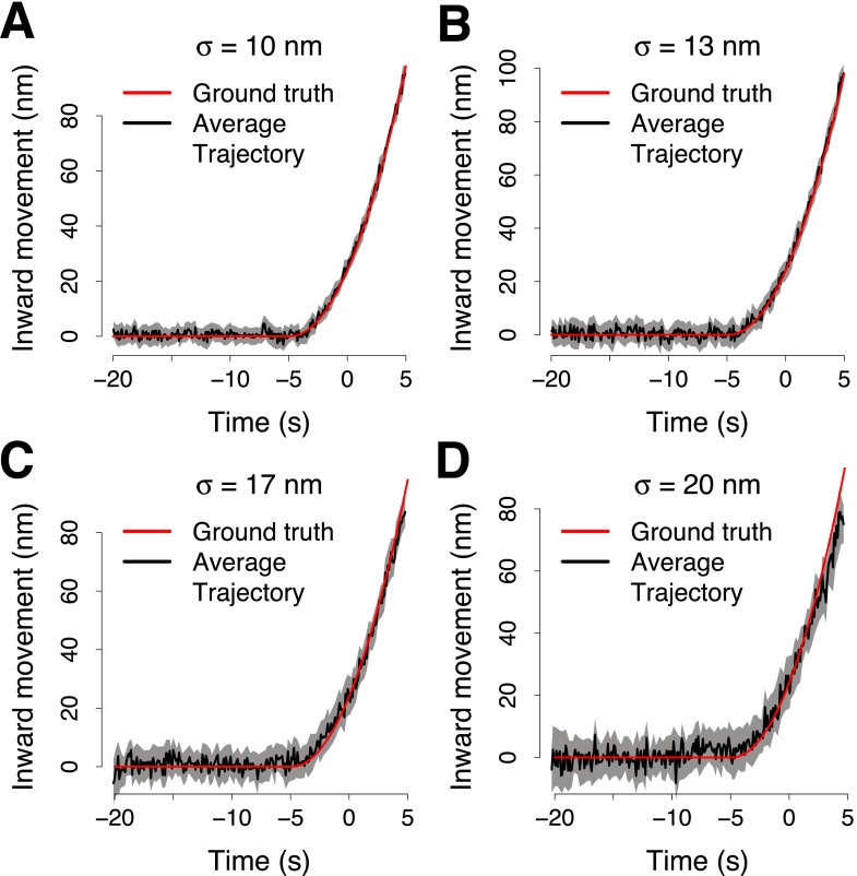
Figure 1u2014figure supplement 5.
Simulation of the accuracy of the trajectory averaging.
( A ) The average trajectory computed from 65 virtual trajectories that were generated from a trajectory template (ground truth trajectory, shown in red) adding noise normally distributed around the p...
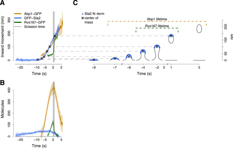
Figure 2.
Alignment of trajectories and interpretation.
( A ) Abp1-GFP, GFP-Sla2 and Rvs167-GFP average trajectories aligned with each other. ( B ) The average number of molecules recruited at the endocytic locus varies from protein to protein, ranging fro...
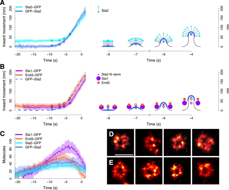
Figure 3.
Coat dynamics and organization.
( A ) Left panel: the inward movement of Sla2 coat protein, tagged at its N- or C-terminus (GFP-Sla2 and Sla2-GFP respectively). Right panel: our model of Sla2 organization at the tip of the plasma me...
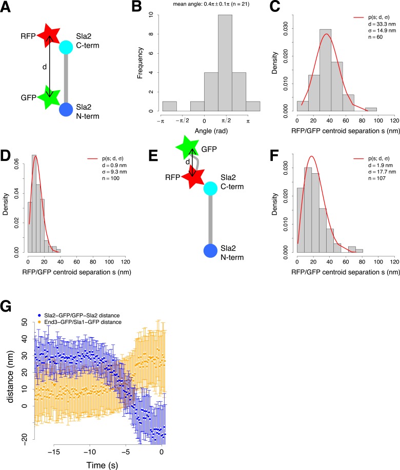
Figure 3u2014figure supplement 1.
Organization of the coat and experimental control for the two color alignment.
( A ) Sla2 N- and C-termini were tagged simultaneously with green (GFP) and red (RFP) fluorescent proteins respectively (GFP-Sla2-RFP). The estimated distance d between the GFP and RFP centroids gives...
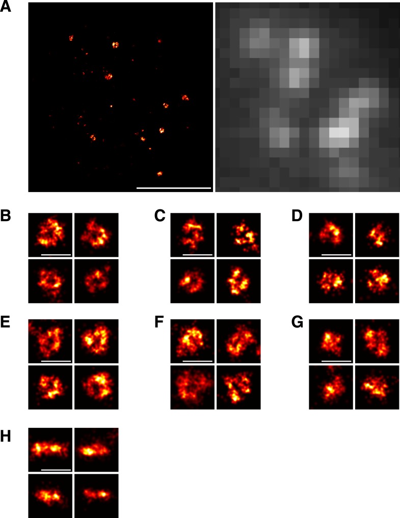
Figure 3u2014figure supplement 2.
Imaging of Sla1 assemblies by localization microscopy.
( A ) Overview of a yeast cell expressing Sla1-SNAP imaged using localization microscopy (left) and conventional, diffraction-limited wide-field microscopy (right). The dashed lines represent the cell...
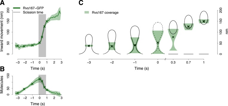
Figure 4.
BAR protein dynamics.
( A ) The inward movement of Rvs167-GFP. ( B ) The average number of molecules of Rvs167-GFP. ( C ) Our model of Rvs coverage of the plasma membrane invagination during the invagination growth. When s...
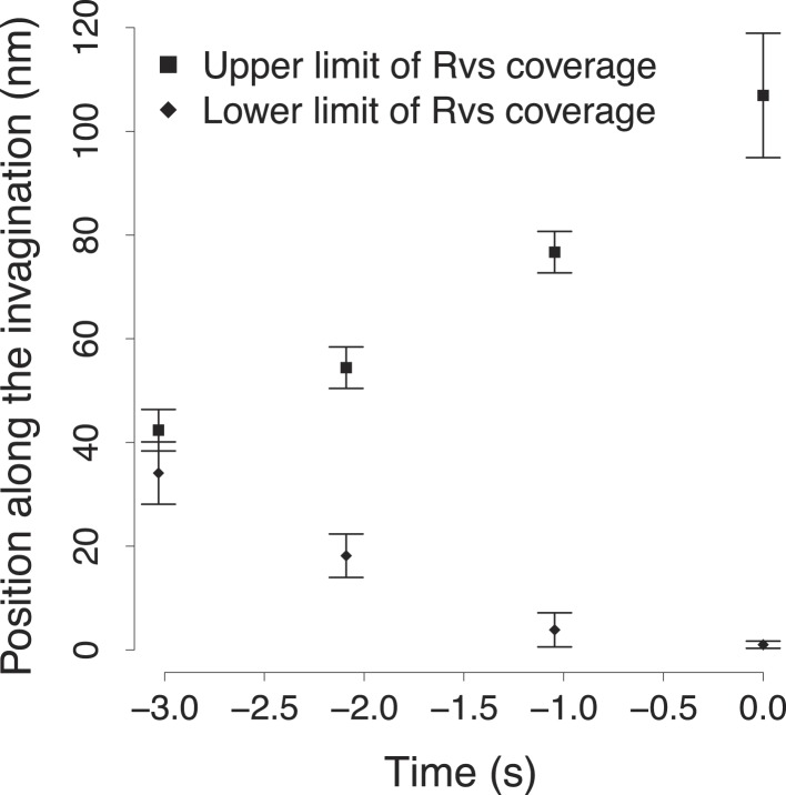
Figure 4u2014figure supplement 1.
The variability in the BAR protein coverage of the plasma membrane.
The points show the upper and lower bound of the Rvs coverage shown in Figure 4C . The error bars show the variability in the calculation of the extent of Rvs coverage of the plasma membrane as a func...
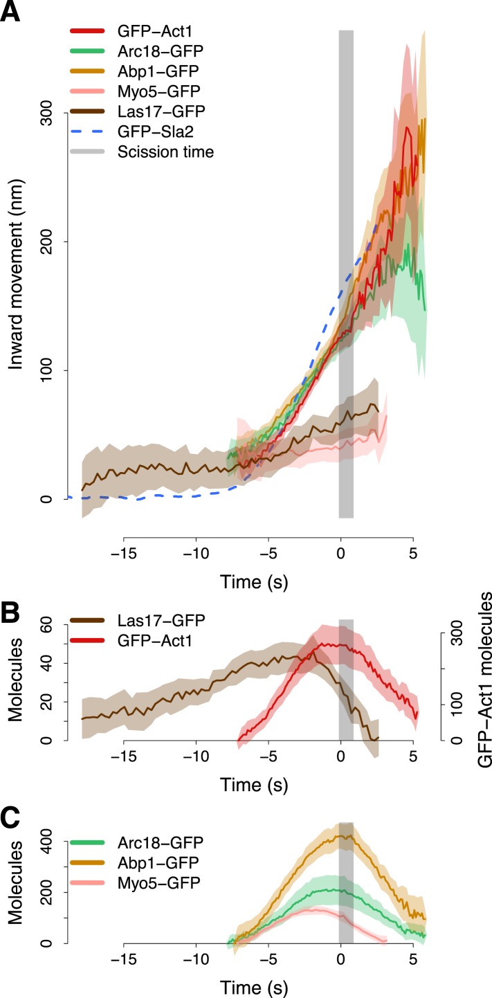
Figure 5.
Actin cytoskeleton dynamics.
( A ) The inward movement of the actin cytoskeleton components GFP-Act1, Arc18-GFP and Abp1-GFP, together with the nucleation factors Las17-GFP and Myo5-GFP. GFP-Sla2 (dashed line) is plotted for comp...
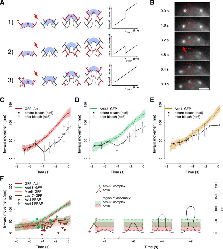
Figure 6.
Region of assembly of actin filaments.
( A ) A schematic cartoon to show how local photobleaching would affect the centroid position of a fluorescent actin patch, given three possible scenarios for the nucleation of new actin filaments (in...
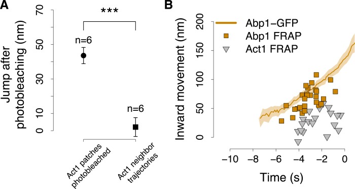
Figure 6u2014figure supplement 1.
The position of Abp1 fluorescence recovery after photobleaching.
( A ) The quantification of the jump in GFP-Act1 patches photobleached 3u20134 s after the appearance of the patch (data showed in Figure 6C ), compared with the jump in GFP-Act1 patches that where ne...
Video 1.
Photobleaching experiment.
Local photobleaching of an endocytic event in a cell expressing GFP-Act1. The video plays in real time. Scale bar is 2 u00b5m. DOI: http://dx.doi.org/10.7554/eLife.04535.019
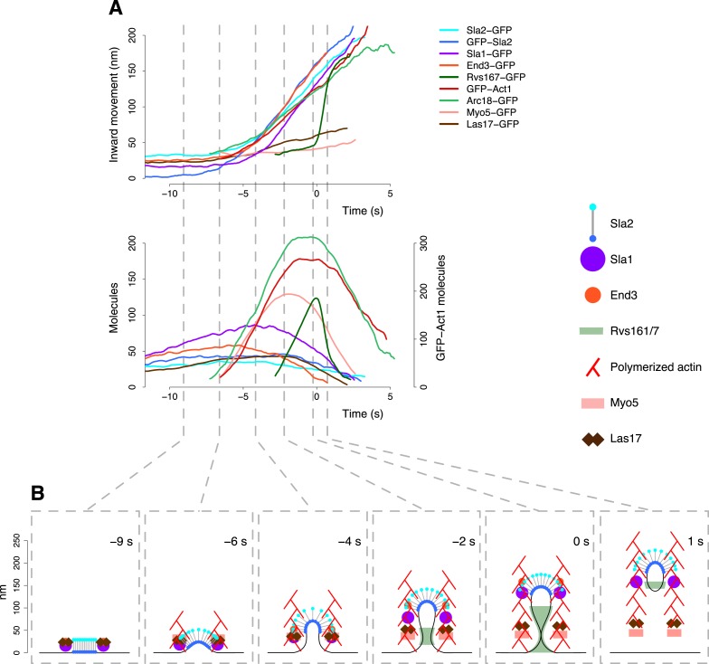
Figure 7.
The dynamic architecture of the endocytic machinery.
( A ) Summary of the average dynamics and number of molecules for Sla2-GFP, GFP-Sla2, Sla1-GFP, End3-GFP, Rvs167-GFP, Arc18-GFP, Myo5-GFP, Las17-GFP and GFP-Act1. The plotted trajectories are listed i...
Video 2.
The dynamic architecture of the endocytic machinery.
The reconstruction of the dynamic architecture of the endocytic machinery obtained by combining the centroid positions of the proteins over time, the plasma membrane invagination profiles derived from...
Figure images are served from the NIH/NLM PubMed Central Open Access Subset or Europe PMC; copyright remains with the publishers and authors.
💬 Discussion
0 commentsNo comments yet. Be the first to start a discussion!
Leave a Comment