Abstract
Abstract The resolution of fluorescence microscopy images is limited by the physical properties of light. In the last decade, numerous super-resolution microscopy (SRM) approaches have been proposed to deal with such hindrance. Here we present Mean-Shift Super Resolution (MSSR), a new SRM algorithm based on the Mean Shift theory, which extends spatial resolution of single fluorescence images beyond the diffraction limit of light. MSSR works on low and high fluorophore densities, is not limited by the architecture of the optical setup and is applicable to single images as well as temporal series. The theoretical limit of spatial resolution, based on optimized real-world imaging conditions and analysis of temporal image stacks, has been measured to be 40 nm. Furthermore, MSSR has denoising capabilities that outperform other SRM approaches. Along with its wide accessibility, MSSR is a powerful, flexible, and generic tool for multidimensional and live cell imaging applications.
🔬 Techniques
🔭 Microscopes
🧬 Organisms
💻 Software
✨ Fluorophores
🧪 Sample Preparation
🔬 Cell Lines
🏭 Microscope Brands
🧪 Reagent Suppliers
📷 Detectors
🔎 Objectives
🎨 Filters
💻 Software Details
💾 Data Repositories
🏷️ Research Resource Identifiers (RRIDs)
Verified research resources used in this paper:
🏛️ Research Organizations (ROR)
Affiliated research institutions:
📋 Methods
Source data availability
All source data used or generated in this study has been made publicly available in the Zenodo OpenAIRE database, and are accessible through a unique DOI, here provided. Dataset title Location DOI Gatta-SIM nanorulers. Fig. 2c . 10.5281/zenodo.6941792 Airyscan and Confocal line pattern. Figs. 3 and 4 . 10.5281/zenodo.6848342 Synapsed homologs of meiotic mouse chromosomes visualized by TIRFM. Fig. 4d . 10.5281/zenodo.6865142 STED immunofluorescence imaging of histone protein H3K27 in a 2-cell stage mice embryo. Fig. 6 . 10.5281/zenodo.6865168 CRISPR-PAINT nanorulers. Fig. 7b–f , Supplementary Figs. S42 – 44 , Supplementary Movie S1 . 10.5281/zenodo.6850637 PSFcheck ring pattern at various SNR. Fig. 8 , Supplementary Figs. S21 – 23 , S25 , S27 – 31 , Supplementary Movies S2 – 3 . 10.5281/zenodo.6955019 Rotavirus viroplasms. Fig. 9a , Supplementary Fig. S32 . 10.5281/zenodo.6850357 Mouse sperm acrosome exocytosis. Fig. 9b , Supplementary Figs. S33 – 34 , Supplementary Movies S4 – 9 . 10.5281/zenodo.6850232 Volumetric imaging of Arabidopsis thaliana root cells. Fig. 9d–e , Supplementary Figs. S39 – 40 , Supplementary Movie S12 . 10.5281/zenodo.6850745 EM-CCD noise image sequence. Supplementary Figs. S16 – 18 . 10.5281/zenodo.6955070 Live-cell imaging of LLC-PK1 cells microtubule dynamics. Supplementary Fig. S37 , Supplementary Movies S10 – 11 . 10.5281/zenodo.6850280 DNA curtain assay for dCas12a/CS10B colocalization. Supplementary Fig. S38 . 10.5281/zenodo.6865120 Volumetric imaging of fluorescently labeled BPAE cells. Supplementary Fig. S41 . 10.5281/zenodo.6865066 Reagents All chemicals were purchased from Sigma-Aldrich Chemical Co. (St Louis, MO) except otherwise indicated. SiR-actin was obtained from Cytoskeleton (Denver, CO) and FM4-64 was purchased from Thermo Fisher Scientific (Waltham, MA). AFM reagents The Acidaminococcus sp dCas12a protein was expressed in Escherichia coli BL21 and purified by chromatography on Ni-NTA (Cytiva), HiTrap SP HP (Cytiva), and HiLoad Superdex 200 16/60 (Cytiva) columns and determined purity through polyacrylamide gel electrophoresis. The 55 nt guide RNA (gRNA) was transcribed in vitro and then purified by TRIzol (Invitrogen) and verified integrity through denaturing urea polyacrylamide gel electrophoresis.
Show full methods section
Source data availability
All source data used or generated in this study has been made publicly available in the Zenodo OpenAIRE database, and are accessible through a unique DOI, here provided. Dataset title Location DOI Gatta-SIM nanorulers. Fig. 2c . 10.5281/zenodo.6941792 Airyscan and Confocal line pattern. Figs. 3 and 4 . 10.5281/zenodo.6848342 Synapsed homologs of meiotic mouse chromosomes visualized by TIRFM. Fig. 4d . 10.5281/zenodo.6865142 STED immunofluorescence imaging of histone protein H3K27 in a 2-cell stage mice embryo. Fig. 6 . 10.5281/zenodo.6865168 CRISPR-PAINT nanorulers. Fig. 7b–f , Supplementary Figs. S42 – 44 , Supplementary Movie S1 . 10.5281/zenodo.6850637 PSFcheck ring pattern at various SNR. Fig. 8 , Supplementary Figs. S21 – 23 , S25 , S27 – 31 , Supplementary Movies S2 – 3 . 10.5281/zenodo.6955019 Rotavirus viroplasms. Fig. 9a , Supplementary Fig. S32 . 10.5281/zenodo.6850357 Mouse sperm acrosome exocytosis. Fig. 9b , Supplementary Figs. S33 – 34 , Supplementary Movies S4 – 9 . 10.5281/zenodo.6850232 Volumetric imaging of Arabidopsis thaliana root cells. Fig. 9d–e , Supplementary Figs. S39 – 40 , Supplementary Movie S12 . 10.5281/zenodo.6850745 EM-CCD noise image sequence. Supplementary Figs. S16 – 18 . 10.5281/zenodo.6955070 Live-cell imaging of LLC-PK1 cells microtubule dynamics. Supplementary Fig. S37 , Supplementary Movies S10 – 11 . 10.5281/zenodo.6850280 DNA curtain assay for dCas12a/CS10B colocalization. Supplementary Fig. S38 . 10.5281/zenodo.6865120 Volumetric imaging of fluorescently labeled BPAE cells. Supplementary Fig. S41 . 10.5281/zenodo.6865066 Reagents All chemicals were purchased from Sigma-Aldrich Chemical Co. (St Louis, MO) except otherwise indicated. SiR-actin was obtained from Cytoskeleton (Denver, CO) and FM4-64 was purchased from Thermo Fisher Scientific (Waltham, MA). AFM reagents The Acidaminococcus sp dCas12a protein was expressed in Escherichia coli BL21 and purified by chromatography on Ni-NTA (Cytiva), HiTrap SP HP (Cytiva), and HiLoad Superdex 200 16/60 (Cytiva) columns and determined purity through polyacrylamide gel electrophoresis. The 55 nt guide RNA (gRNA) was transcribed in vitro and then purified by TRIzol (Invitrogen) and verified integrity through denaturing urea polyacrylamide gel electrophoresis.
Antibodies
The following list of antibodies was used in this study: Mouse monoclonal antibody VP4 (2G4) (Harry B. Greenberg, Stanford University. PMID: 2431540 ). Dilution 1:1000. Mouse monoclonal antibody VP7 (M60) (Harry B. Greenberg, Stanford University. PMID: 2431540 ). Dilution 1:2000. Mouse monoclonal antibody VP7 (159) (Harry B. Greenberg, Stanford University. PMID: 2431540 ). Dilution 1:2000.
Mouse polyclonal antibody NSP2
(Made by our laboratory, PMID: 9645203 ; RRID: AB_2802096 ). Dilution 1:100. Rabbit polyclonal antibody NSP2 (Made by our laboratory, PMID: 9645203 ; RRID: AB_2802097 ). Dilution 1:2000. Rabbit polyclonal antibody NSP4 (Made by our laboratory, PMID: 18385250 ; RRID: AB_2802094 ). Dilution 1:1000. Rabbit polyclonal antibody NSP5 (Made by our laboratory, PMID: 9645203 ; RRID: AB_2802098 ). Dilution 1:2000. Goat anti-rabbit Alexa 568 (Invitrogen, A-11011 ). Dilution 1:10000. Goat anti-mouse Alexa 488 (Invitrogen, A-10680 ). Dilution 1:10000. Primary mouse anti-H3K27me (Abcam, ab6002 ). Dilution 1:200. Primary rabbit anti-H3K27ac (Active Motif, 39034 ). Dilution 1:200. Secondary goat anti-mouse STAR Red (Sigma-Aldrich, 52283 ). Dilution 1:500. Secondary goat anti-rabbit STAR Orange (Sigma-Aldrich, 41367 ). Dilution 1:500. Secondary anti-mouse Alexa 568 (Thermo, A11004 ). Dilution 1:400. Primary SCP-3 (D-1) antibody (Santa Cruz Biotechnology, SC-74569 ). Dilution 1:300. Monoclonal ANTI-FLAG ® BioM2-Biotin (Sigma-Aldrich, F9291 ) conjugated to quantum dots (Thermo, Q21361MP ). Dilution 1:66665.
Animals
CD1 mature (10- to 12-week old) male mice were used. Animals were maintained at 23 °C and 55 ± 15% humidity, with a 12-h light—12-h dark cycle. Water was always accessible. Animal and plant experimental procedures treated at the Instituto de Biotecnología (IBt) were approved by the Bioethics Committee of the Instituto de Biotecnología of the Universidad Nacional Autónoma de México (UNAM). Animal experimental procedures treated at the Department of Biomedicine and Prevention at Faculty of Medicine were approved by the “Ministero della Salute” of Italy, authorization n.701/2018-PR.
Animal experimental procedures treated on the Neurobiology and Epigenetics
Unit of the European Molecular Biology Laboratory were approved by the EMBL Rome Animal Facility in accordance with European and Italian legislations. CRISPR/Cas protein expression and purification Nuclease-dead dCas12a from Acidaminococcus sp. (Addgene, #171668) fused to an N-terminal 6His-SUMO tag was expressed in Escherichia coli BL21. Cells were grown in Luria-Bertani broth at 37 °C and transferred to 12 °C when OD600 reached 0.8. After 1 h, IPTG was added to a final concentration of 1 mM. After 24 h growth, cell pellets were collected by centrifugation and stored at −70 °C until protein purification. The pellet was thawed in a lysis buffer (20 mM Tris-HCl pH 8.0, 250 mM NaCl, 10 mM imidazole) and sonicated for 6 min in 5 s ON-25 s OFF intervals. This was followed by centrifugation at 35,000 g at 4 °C for 35 min and filtration using membranes with 0.22μm pore-size. The cell-free extract was injected into a Ni-NTA column (Cytiva) and eluted with an elution buffer: 20 mM Tris-HCl pH 8.0, 1 M NaCl, 250 mM imidazole. The protein was mixed with the SUMO protease and dialyzed overnight at 4 °C in dialysis buffer (50 mM phosphate buffer pH 6.0, 100 mM KCl, 5 mM MgCl 2 , 10% glycerol, 2 mM DTT) to remove the 6His-SUMO tag. The cleaved protein was injected into a cation exchange HiTrap SP HP column (Cytiva) and eluted with a linear gradient from 0 to 50% IEX buffer (20 mM HEPES-KOH pH 7.2, 100 mM KCl, 5 mM MgCl 2 , 10% glycerol, 2 mM DTT). The protein was further purified by size exclusion chromatography on a HiLoadSuperdex 200 pg 16/60 column (Cytiva) in storage buffer (20 mM HEPES-KOH pH 7.5, 500 mM KCl, 10% glycerol) and aliquots were stored at −70 °C until use. Purity and identity of dCas12a were confirmed via polyacrylamide gel electrophoresis and western-blot against the 6xHis region on dCas12a. Methods used for Supplementary Fig. S38 .
Production of crRNAs The crRNA used in atomic force microscopy
(AFM) experiments (Supplementary Fig. S42b ) was produced by in vitro transcription of DNA templates previously amplified by PCR. The templates were produced using two self-complementary oligos (purchased from IDT). Fw 5′-GAAATTAATACGACTCACTATAGGTAATTTCTACTCTTGTAGAT-3′ and Rv 5′-CCCTGGTCAACCAGGTGAACAAGGATCTACAAGAGTAGAAATT-3′. In vitro transcription and crRNA purification were performed using HiScribe T7 (NEB, E2040S) and RNA Cleanup (NEB, T2040S) kits, respectively. The crRNA pool for DNA curtains was produced according to the following procedure. Partially double stranded DNA templates for in-vitro transcription were obtained by hybridizing a 24 nt long forward oligo encoding the promoter for T7 RNA polymerase: 5′ GAAATTAATACGACTCACTATAGG, with a pool of five 68 nt long reverse oligos (purchased from IDT): 5′-AUGAUGUUCUGCUGGAUAUGCACU-3′, 5′-CCUGACACCGGACGGAAAGCUGAC-3′, 5′-AAUGUCGGCUAAUCGAUUUGGCCA-3′, 5′-GCUAGCAAUUAAUGUGCAUCGAUU-3′ and 5′-AUGAACGCAAUAUUCACAAGCAAU-3′, which encoded the crRNA sequence and the region complementary to the T7 promoter. Forward and reverse oligos were annealed at 1.5:1 ratio (Fw:Rv) in 10 mM Tris-HCl, pH 7.5, 50 mM NaCl, 1 mM EDTA buffer, incubated at 75 °C for 5 min and cooling to 25 °C during 25 min. HiScribe T7 kit was used for in vitro transcription and the crRNA pool was purified with TRizol (Ambion). Methods used for Supplementary Fig. S38 . CRISPR/dCas12a nanoruler preparation First, the CRISPR/dCas12a ribonucleoprotein (RNP) complex was formed. On a 0.6 mL microcentrifuge tube, the following reagents were added (final concentration): 1× CRISPR action buffer (TRIS-HCl 200 mM, NaCl 500 mM, DTT 5 mM) and dCas12a 20 nM. The gRNA was pre-heated at 90 °C for 1 min and then let cool to room temperature. Upon gRNA cooling, it was added to the dCas12a to a final concentration of 30 nM. The CRISPR/dCas12a components were incubated for 20 min at room temperature. When the complex was formed, the target dsDNA was added and the microtube was incubated at 37 °C for 1 h so the CRISPR/dCas12a complex binds to the target sequences in the dsDNA and thus forms the CRISPR/dCas12a nanoruler. Methods used for Supplementary Fig. S38 . CRISPR/dCas12a nanoruler slide preparation for fluorescence microscopy The sample imaging volume was delimited by a perforated double-sided tape attached to a coverslip and a slide on each side. The following reagents were prepared on an independent microtube: CRISPR/dCas12a nanorulers (described in the previous section), 20 μg/mL Hoechst33342, and 5 nM ssDNA fluorescent probe PS3 88 (5′-TCCTCCC-3′-ATTO 647 N, Integrated DNA Technologies’) and graded with ddH 2 O. The mix was transferred to the perforated double-sided tape in the coverslip and covered with the slide. The following sequence represents the dsDNA used for CRISPR/dCas12a binding, in which bold sequences corresponds to the association sites and italics are the protospacer adjacent motif (PAM) sequence: AATTCTTAGGCACCCTTCTTTTTCTTCTTCTTCTTTTTCTTCTTTTTCTTAGCACCTTGGCCGGCTCCAGCACCGGCTCCTTGACCAGCACCAGCACCAGCACCTTGGCCGGCTCCAGCACCGGCTCCTTGACCAGCACCAGCACCAGCACCTTGGCCGGCTCCAGCACCGGCTCCTTGACCAGCACCAGCACCAGCACCTTGGCCGGCTCCAGCACCGGCTCCTTGACCAGCACCAGCACCAGCACCTTGGCCGGCTCCAGCACCGGCTCCTTGACCAGCACCAGCACCAGCACCAGCACCGGCTGGACCCTGGTTTCCTGG TTTA CCTTGTTCACCTGGTTGACCAGGG TTACCTGGCTGACCAGGGGAACCTTGGTTACCTGGAGAGCCTTGTGAACCTGGGGATCCAGGTTGACCATTCTTTCCAGGGTTACCCTGAGAACCTTGTGGACCGTTGGAACCTGGCTCACCAGGTTGTCCGTTCTGACCAGGTTGACCAGGTTGACCTTCGTTTCCTGGTTGACCTGGATTACCTGGAGAACCCTTGTTACCGGGCTGTCCTTGGTTACCAGGAGATCCTGGGTTACCTGGCTCACCGGCTGGACCCTGGTTTCCTGG TTTA CCTTGTTCACCTGGTTGACCAGGG TTACCTGGCTGACCAGGGGAACCTTGGTTACCTGGAGAGCCTTGTGAACCTGGGGATCCAGGTTGACCATTCTTTCCAGGGTTACCCTGAGAACCTTGTGGACCGTTGGAACCTGGCTCACCAGGTTGTCCGTTCTGACCAGGTTGACCAGGTTGACCTTCGTTTCCTGGTTGACCTGGATTACCTGGAGAACCCTTGTTACCGGGCTGTCCTTGGTTACCAGGAGATCCTGGGTTACCTGGCTCACCGGCTGGACCCTGGTTTCCTGG TTTA CCTTGTTCACCTGGTTGACCAGGG TTACCTGGCTGACCAGGGGAACCTTGGTTACCTGGAGAGCCTTGTGAACCTGGGGATCCAGGTTGACCATTCTTTCCAGGGTTACCCTGAGAACCTTGTGGACCGTTGGAACCTGGCTCACCAGGTTGTCCGTTCTGACCAGGTTGACCAGGTTGACCTTCGTTTCCTGGTTGACCTGGATTACCTGGAGAACCCTTGTTACCGGGCTGTCCTTGGTTACCAGGAGATCCTGGGTTACCTGGCTCACCGGCTGGACCCTGGTTTCCTGG TTTA CCTTGTTCACCTGGTTGACCAGGG TTACCTGGCTGACCAGGGGAACCTTGGTTACCTGGAGAGCCTTGTGAACCTGGGGATCCAGGTTGACCATTCTTTCCAGGGTTACCCTGAGAACCTTGTGGACCGTTGGAACCTGGCTCACCAGGTTGTCCGTTCTGACCAGGTTGACCAGGTTGACCTTCGTTTCCTGGTTGACCTGGATTACCTGGAGAACCCTTGTTACCGGGCTGTCCTTGGTTACCAGGAGATCCTGGGTTACCTGGCTCACCGGGTGCACCAGCACCGAGACCACAAGCTTCAGCTTCTCTCTTCTCGAGAGAT 3′. Methods used for Supplementary Fig. S38 . GATTA-PAINT and CRISPR/dCas12a nanoruler sample imaging The GATTA-PAINT 40 RG nanoruler was provided as a single slide ready for imaging (GATTAquant DNA nanotechnologies). It has three fluorophores at a separation of 40 nm between them (ATTO 542/ATTO 655) and 80 nm between the furthest. Imaging was performed on an Olympus IX-81 inverted microscope using total internal reflection fluorescence (TIRF) illumination with a penetration depth of 200 nm (Olympus, cellTIRF Illuminator). Images were collected with an iXon 897 EMCCD camera (Model No. DU-879-CS0-#BV). A set of 300 frames were acquired at an exposure time of 50 ms per image, excitation laser of 488 and 561 nm with full laser power (23.1 mW measured at the back focal plane of the lens), and an effective pixel size of 160 nm in the object plane (Olympus UApo N 100×/1.49 numerical aperture, oil-immersion). For MSSR only the first 100 frames were analyzed. The CRISPR/dCas12a nanoruler sample was visualized on the same imaging setup as the GATTA-PAINT 40RG nanoruler, except that a 20 ms as acquisition time was employed. Nearby emitters were automatically identified from t-MSSR 3 -Var images using the Maximum Finder function of FIJI/ImageJ. A Maxima was accepted only if its intensity value (digital gray levels) was higher than a threshold value (prominence = 1900), in comparison with the intensity values from the ridge to a higher maximum. The coordinates of the identified local maxima (emitter’s location) were computed from 16 regions of interest (1.5 µm 2 each) and exported to R to further quantify the intermitter’s distances considering a worm-like chain model 48 . Briefly, the intermitter distances were computed for any pair of identified local maxima within the same t-MSSR 3 -Var image. The CRISPR/dCas12a nanoruler system was design to with four binding sites for dCas12a distributed uniformly every 297 bp (equivalent to ~100 nm), hence, two emitters are considered to be part of the same dsDNA if their intermitter distance is shorter than the accumulated distance of four binding sites (300 nm). All measured intermitter distances were pooled on a single histogram and fitted in the context of Gaussian mixture models. Fitting was performed in R with the normalmixEM routine of mixtools with parameters µ: {µ 1 = 100, µ 2 = 200, µ 3 = 300} nm, and σ = sqrt(µ). Multiple fields of GATTA-PAINT and CRISPR/dCas12a nanorulers were imaged with similar results, but only one representative dataset for each sample is showcased in Fig. 7 . Methods used for Fig. 7 , Supplementary Fig. S43 and Supplementary Movie S1 . AFM visualization The RNP particle was assembled from dCas12a and crRNA (1:1.5 molar ratio) in AFM buffer (20 mM Tris-HCl pH 8.0, 100 mM NaCl, 15 mM MgCl 2 , 1 mM DTT) at 37 °C for 20 min. The DNA template (1,500 bp) with four dCas12a target sites was added to the mix at 40:1 (RNP:DNA) molar ratio and incubated for 1 h at 25 °C. The sample was diluted 5-fold to a final concentration of 1 nM DNA and deposited on a freshly cleaved mica for 10 min, followed by rinsing with 0.5 mL filtered milli-Q water and air-drying. Images were acquired with an atomic force microscope (NanoScope V, Bruker) on ScanAsyst-Air mode at room temperature and 1,024 samples/line. Images were processed with NanoScope Analysis Software v1.89. Methods used for Supplementary Fig. S42b . This experiment was performed once.
DNA curtain assay
DNA from bacteriophage λ (λDNA) (NEB, N3011S) was mixed with biotinylated oligos complementary to the cohesive ends of λDNA in reaction buffer for T4 DNA ligase (NEB, M0202S), incubated at 70 °C for 15 min and cooled down to 15 °C, over 2 h. T4 DNA ligase was used for overnight ligation at room temperature. After ligase inactivation with 2 M NaCl, the biotinylated DNA was purified on a Sephacryl S-1000 size exclusion column (GE Healthcare). The flowcell was passivated with a lipid solution (1.954% DOPC, 0.04% DOPE-mPEG2k and 0.006% DOPE-biotin) in buffer (10 mM Tris-HCL pH 8, 100 mM NaCl) for 30 min at room temperature. The flowcell was washed with BSA buffer (40 mM Tris-HCl pH 8, 2 mM MgCl 2 , 0.2 mg/mL BSA) and incubated for 10 min. The biotinylated DNA in BSA buffer was injected into the flowcell and non-tethered DNA was washed out. BSA buffer supplemented with 100 mM NaCl, 5 mM MgCl 2 , 2 mM DTT was used for imaging. RNP particles were prepared by mixing dCas12a with the crRNA pool at 1:10 molar ratio in buffer (20 mM Tris-HCl pH 8.0, 100 mM NaCl, 5 mM MgCl 2 , 2% glycerol, 2 mM DTT) at 37 °C for 30 min. The complex (10 nM) was injected into the flowcell for DNA binding during 30 min at room temperature. Labeling of dCas12a was achieved with anti-FLAG antibodies conjugated to quantum dots (Thermo, Q21361MP). C-S10-B was labeled with maleimide-Alexa488 at a single N-terminal cysteine. Images were acquired at 60× with an inverted Nikon Ti-E microscope with 488 nm excitation laser. Emission was split with a 638 nm dichroic beam splitter (Chroma) and captured by two EM-CCD cameras (Andor iXon DU897). Images were processed with FIJI 89 . Methods used for Supplementary Fig. S38 . Structured-illumination microscopy The GATTA-SIM 140B nanoruler was provided as a single slide ready for imaging (GATTAquant DNA nanotechnologies). Spreads of germ cell chromosomes were performed according to Faieta 90 . In brief, testes were removed from euthanized animals, decapsulated, macerated in high-glucose MEM and mixed. The suspension was left to settle, and the supernatant was spun down at 7200 rpm for 1 min. The pellet was resuspended in 0.5 M sucrose and the suspension was added to slides coated with 1% paraformaldehyde in 0.015% Triton X-100 and incubated for 2 h in a humidified chamber at room temperature. At the end of the incubation, slides were rinsed twice in 1:250 Photo-Flo (Kodak, 1464510) in water and allowed to air dry. Surface chromosome spreads were either immediately processed for immunofluorescence or stored at −80 °C for up to 6 months. SYCP3 was stained using a primary antibody from Santa Cruz SC-74569 (SYCP3 D1) and a secondary antibody anti-mouse Alexa 568 (Thermo, A11004). Imaging of both the nanorulers and the mouse chromosomes was performed using an Elyra 7 microscope (Zeiss). Image acquisition was made with a 60 × 1.4 NA oil immersion objective and a 1.4× lens as extra magnification. Image reconstruction was done in ZEN Black with default parameters. Both the experiments involving the GATTA-SIM nanorulers and mouse germ cell chromosomes were performed once to obtain representative datasets. Methods used for Figs. 2 c and 4d . Rotavirus cell infection and viral replication machinery immunofluorescence imaging MA-104 Clone 1 cells (American Type Culture Collection; ATCC: CRL-2378.1 ; RRID: CVCL_3846 ) were cultured in DMEM-RS media supplemented with 5% fetal bovine serum at 37 °C and 5% CO 2 . Prior to infection, Rhesus rotavirus (RRV) was activated with trypsin (10 μg/ml) for 30 min at 37 °C. MA104 cells grown on glass coverslips were infected with RRV at a multiplicity of infection (MOI) of 1 54 . At six hours post infection, the cells were fixed and processed for immunofluorescence. The coverslips were mounted onto the center of glass slides with a STORM buffer mounting medium (1.5% glucose oxidase + 100 mM β-mercaptoethanol). All images were kindly provided by Garcés and collaborators 54 . Briefly, images of the rotavirus viroplasm were acquired on an Olympus IX-81 inverted microscope configured for total internal reflection fluorescence (TIRF) excitation (Olympus, cellTIRFM illuminator) using a critical angle such that the evanescence field had a penetration depth of 200 nm. The fluorophores Alexa Fluor 488 and Alexa Fluor 568 were excited with light of 488 nm and 568 nm respectively. The optical setup consists of an Olympus UApo N 100×1.4 NA, oil-immersion objective lens, with an extra 1.6× intermediate magnification lens. The images were acquired by an EMCCD camera (iXon 897, Model No: DU-897E-CS0-#BV; Andor) at a frequency of 20 fps and effective pixel size of 100 nm at the object plane. MSSR processing was performed considering the following parameters: AMP = 5, PSF = 3, order = 1. GPU parallel computing was enabled, and 100 images were used with t-MSSR-Mean. Methods used for Fig. 9a and Supplementary Fig. S32 . Note: ATCC:CRL-2378 cells were discovered to be contaminated with cells of African Green Monkey (AGM) origin. MA-104 was developed by initial explant culture from embryonic Rhesus Monkey kidney tissue. The cells were deposited at early passage to ATCC in the 90 s, and, after extended passage at ATCC, isoenzymology detected AGM cells. Observations suggest that the Rhesus Monkey cells were completely overtaken by the AGMs between passage 7 and 12. A pure population of Rhesus Monkey cells could not be obtained from the original deposit, and CRL-2378 was discontinued from the collection. However, the AGM subpopulation was cloned out, expanded and preserved as MA-104 Clone 1 (ATCC CRL-2378.1). Live imaging of sperm acrosomal exocytosis and F-actin dynamics The non-capacitating medium (NC) used was a modified Toyoda–Yokoyama–Hoshi (modified TYH) which contains 119.3 mM NaCl, 4.7 mM KCl, 1.71 mM CaCl 2 .2H 2 O, 1.2 mM KH 2 PO 4 , 1.2 mM MgSO 4 .7H 2 O, 0.51 mM sodium pyruvate, 5.56 mM glucose, 20 mM HEPES and 10 µg/ml gentamicin. For capacitating conditions 15 mM NaHCO 3 and 5 mg/ml BSA were added (CAP). Animals were euthanized and cauda epididymal mouse sperm were collected. Both cauda epididymis were cut at multiple sites and placed in 500 µl of NC. After 15 min incubation at 37 °C the epididymis were removed. Sperm were pre-incubated for 10 min in the presence of 100 nM SiR-actin in NC. Once loaded, sperm were incubated for another 60 min in CAP, the concentration of SiR-actin was 100 nM during the whole experiment. Sperm were immobilized on concanavalin-A (1 mg/ml)-coated coverslips. The chamber was then filled with a recording medium (NC) containing 100 nM SiR-actin and 0.5 µM FM4-64. 100 images were obtained every 30 s for 20 min using the NanoImager S microscope (Oxford Nanoimaging Ltd), equipped with a 100×, 1.4 NA, oil-immersion objective (Olympus). For SiR-actin excitation, a 640 nm laser was used and for FM4-64 excitation a 561 nm laser was used. Effective pixel size at object plane = 117 nm. Sperm cells were imaged multiple times with similar results, but only a representative sequence is shown. Methods used for Fig. 9b , Supplementary Figs. S33 – S34 and Supplementary Movies S4 – 9 .
Imaging of Arabidopsis thaliana root cells
Arabidopsis thaliana seeds were surface sterilized, germinated and grown in 0.2× Murashigue and Skoog medium (prepared based on Linsmaier and Skoog medium L477; PhytoTechnology Laboratories, Lenexa, KS, USA), pH 5.7, supplemented with vitamins (0.1 mg l -1 pyridoxine, 0.1 mg l-1 nicotinic acid), 1% sucrose, and 0.8% agar. The plants were grown in a chamber at 21 °C, 16/8 h light/dark photoperiod and a light intensity of 105 µmol photons m −2 s −1 . Confocal imaging of the double transgenic line, an F1 of a cross between plasmalemma pUBQ10::NPSN12-YFP 70 and nuclear p35S:H2B:RFP 91 marker lines, was performed with a Zeiss Axiovert 200 M microscope equipped with a C-APO ×63, 1.2NA objective (Oberkochen, Germany) and a coupled confocal system with a 488-nm laser source, a filter cube with 525/45 nm and 630/92 nm bandpass filters for yellow and red fluorescent protein emission, respectively, and a linear motor travel XY Stage and a Z-axis piezo stage with controllers (Thorlabs, Inc. Newton, NJ, USA). The XY pixel size of 404 nm and Z step size of 500 nm were implemented. Supplementary Fig. S39a–c show a Z-projection (sum) of ten slices, with the red and green channels represented by the “Cyan Hot” and “Magenta” look-up tables (LUTs), respectively. A nuclear marker line, p35S:H2B:RFP, was imaged with an inverted Olympus FV1000-IX81 confocal microscope equipped with a LUMFLN×60, 1.3NA S objective. The 543 nm laser was used to excite RFP and emitted light was filtered with BA560–660. The oversampled XY pixel size of 41 nm and Z step size of 100 nm were implemented. The final image in Supplementary Fig. S39d was made by a Z-projection of 86 slices with MAX intensity mode and the LUT used was “Royal” of FIJI 89 . SPIM imaging of A. thaliana root cells was performed over a transgenic primary root expressing p35s:H2B-R with an in-house SPIM system inspired on the OpenSPIM project 92 , with some setup modifications of the original design. Briefly, the illumination path consists of a C-flex laser combiner providing laser excitation sources at 405, 488, 561, 638 nm (Hubner Photonics, Cobolt Series 01–06, DPL for 561 and MDL for 405,488,638), which is coupled to the SPIM optics through a single multimode laser guide (Fiber optic with FC-APC output). Laser light is focused on a horizontal plane shaped via cylindrical lens (Thorlabs ACY254-050-A, f = 50.0 m ± 1%, Ø 25.4 mm, AR Coating: 350 − 700 nm). The focal plane of the cylindrical lens is imaged by a telescope in the back focal plane of the illumination objective (Olympus UMPLFLN10XW, 10X water immersion, NA = 0.3 mm WD = 3.5 mm). The excitation light-sheet is confined within the imaging area by a slit (Thorlabs VA100/M, Adjustable Mechanical Slits, Internal thread =2.4 mm), which is placed in the center of the telescope. The resulting light-sheet has a beam waist of about 3 µm in the focal plan of the illumination objective. The detection unit consists of a 20× water immersion objective (Olympus UMPLFLN20XW, NA = 0.5 mm WD = 3.5 mm), a tube lense (Ø60 mm × 104 mm), a multi-bandpass emission filter set (Semrock, FF01-446/523/600/677-25 BrightLine, Ø25 mm × 3.5 mm), and a sCMOS camera (Hamamatsu, ORCA-Flash4.0 V2 - Camlink 100fps). A 3D printed water filled imaging chamber (internal volume = 22 × 22 × 30mm without objectives) embodies the illumination objective and the detection objective aligned at 90°, a custom-made 3D printed sample holder and the sample. Fluorescence excitation of the H2B-R-RFP expressing root cells was provided via the 561 nm laser light using stroboscopic illumination. SPIM volumetric imaging was achieved by mounting the sample on a four dimensional (XYZ, and Y rotation) motorized stacked stage (Picard Industries, USB 4D Stage, linear range = 9 mm, Includes Sample-Arm). Computer control of stroboscopic illumination, image acquisition and sample translation were provided by the OpenSPIM plugin 64-Bits of µmanager (v.1.4 for windows) 93 . Images were collected at a final pixel size of 0.325 µm, a z-step of 1.524 µm and a rotation step of 1.8°. MSSR processing was performed considering the following parameters: AMP = 10, PSF = 2, order = 0. Imaging of A. thaliana root cells was performed repeatedly but only one representative experiment was showcased. Methods used for Fig. 9d–e , Supplementary Figs. S39 and S40 and Supplementary Movie S12 . Volumetric imaging of BPAE cells FluoCells™ Prepared Slide #1 (BPAE cells with MitoTracker™ Red CMXRos, Alexa Fluor™ 488 Phalloidin, and DAPI, Thermo, # F36924 ) were imaged using the Nanoimager-S microscope (Oxford Nanoimaging Ltd), with a 100×, 1.4 NA, oil-immersion objective (Olympus) with and a sCMOS camera (Hamamatsu, ORCA-Flash4.0 V2 - Camlink 100fps). For DAPI, Alexa Fluor™ 488 phalloidin and MitoTracker™ Red CMXRos excitation, 405 nm, 473 nm and 561 nm lasers were used, respectively (Channel Splitter dichroic 561 LP. Emission Filter 1: 525/50, Emission Filter 2: Band 1 575–616.5). A set of 22 images (33 ms) were collected as a z-stack for each channel. Each frame was collected with a separation in z of 50 nm. Imaging of BPAE cells was performed several times but only one representative experiment was showcased. Methods used for Supplementary Fig. S41 and Supplementary Movies S13 and S14 . Live-cell imaging of LLC-PK1 cells microtubule dynamics LLC-PK1 (ATCC: CL-101 ) cells stably expressing mEmerald-EB3 were cultured and imaged using an ORCA-Fusion back-thinned sCMOS camera (Hamamatsu, C15440-20UP) and a 100×/1.47 NA oil-immersion objective (Plan-Apochromat, Zeiss) in a Zeiss Celldiscoverer 7 microscope with CO 2 and temperature control set at 5% and 37 °C, respectively. Fluorescence excitation was provided by a 488 nm laser at 1% laser power and emission light (λ em = 510 nm) was collected using a FITC filter. Image collection was done using the ZEN 3.2 (blue edition) acquisition software, with an exposure time of 100 ms, 2 s −1 frame rate and a 43 nm pixel size. Stable cell lines were generated and provided by Michael W. Davidson 94 , 95 . Imaging of LLC-PK1 cells was performed repeatedly but only one representative experiment was showcased. Methods used for Supplementary Fig. S37 and Supplementary Movies S10 and S11 .
STED microscopy
Immunofluorescence imaging was carried out using a STEDYCON mounted on an upright Zeiss microscope in confocal or STED modes. Samples were imaged with a Zeiss 100×1.46 NA objective, 20 nm pixel size, 5 µs pixel dwell time, 15-line accumulations and a pinhole of 64 µm. Immunofluorescence was performed as in 45 . Primary antibodies used were anti-H3K27me (Abcam ab6002) and anti-H3K27ac (Active Motif, 39034), both at 1:200 dilution. Secondary antibodies used were anti-mouse labeled with STAR Red and anti-rabbit labeled with STAR Orange. STED laser powers were 3% of the 640 nm and 775 nm 96.5% for the STAR red channel, whereas for the STAR Orange channel was 7.8% of the 561 nm laser and 100% for 775 nm. Multiple cells were imaged with similar results but only one representative experiment was showcased. Methods used for Fig. 6 . ArgoLight “Argo-SIM“ test slide Confocal images were acquired on a Zeiss LSM880 inverted microscope using a Plan-Apochromat 63×/1.4 Oil immersion objective, exciting the micropattern with the laser 405 nm and detecting the fluorescence in the range 420–480 nm. The pixel size was 0.044 micrometers. The same area has been acquired using the Airyscan detector with the same settings for laser power, detector gain, image format, bit depth, and line averaging, using a selective optical filter BP 420–480 + LP 605, and processing the images with the Airyscan algorithm (Zen Black, AIMApplication version 14.0.22.201) with strength parameter set to 6. Methods used for Fig. 4 .
PSFcheck imaging
We employed an immobile fluorescence pattern as a calibration sample for SRM 53 . The fluorescent patterns were fabricated using direct laser writing via infrared ultrashort-pulses that create regions of autofluorescence in a two-part epoxy mixture polymer sandwiched between a coverslip and a microscope slide (PSFcheck). One of the patterns present on a PSFcheck calibration slide consists of a 3D array of small diffraction limited shell features separated 10 µm from each other. The fluorescent thickness of a shell is small compared to the PSF so that the average FWHM across several features was calculated to be of 208 nm in a SIM microscope. We imaged this shell pattern using widefield fluorescence excitation on a NanoImager-S (Oxford Nanoimaging Ltd), equipped with a 100×, 1.4 NA, oil-immersion objective (Olympus). The PSFcheck sample was excited with a 561 nm laser and the emitted fluorescence acquired in the Emission Filter 2: Band 1 575–616.5 and recorded on a sCMOS Hamamatsu Orca Flash 4.0 V3. Acquisition time = 33 ms, effective pixel size at object plane = 117 nm. Imaging of the PSFcheck pattern was done once. Methods used for Fig. 8 , Supplementary Figs. S21 – 23 , S25 , S27 – 31 , and Supplementary Movies S2 and S3 . ORCA Flash 4.0 V3 sCMOS detector characterization and Automatic Correction of sCMOS-related Noise (ACsN) The fixed noise patterns of a sCMOS detector characterize the offset, variance and gain of each pixel in so-called calibration maps. The offset and variance are the average and variance, respectively, of the digital pixel-wise values that result from a video where no photons hit the detector. The gain is a multiplicative value of the signal when photons are detected. To characterize the maps of the sCMOS ORCA Flash 4.0 V3 detector, a code was written in the R programming language that implements the previously described calibration 96 . For the calculation of the offset and variance, a video of 60 thousand images was acquired without illumination on the NanoImager-S microscope (Oxford Nanoimaging Ltd) with no sample or laser turned on. In addition, a uniform fluorescent sample was used to recreate a uniform illumination of the detector and 5 videos of one thousand images each were taken. Each video had an average number of photons, chosen to be between 20 and 200 photons per pixel with even increments between each consecutive video as described by Huang et al. ACsN is a noise correction method for sCMOS images that uses a principle of similarity between patches within the same image to characterize noise using 3D filtering 97 . The camera noise together with the signal from the incident photons can be represented by a distribution whose standard deviation is approximated based on the frequency thresholds of the modulation transfer function (MTF). This threshold is calculated from the optical parameters of the system. The ACsN application was used in Matlab version 2020a. The input parameters were 1.4 of numerical aperture, wavelength of 610 nm, and pixel size of 117 nm, without video filter and with parallel computation. Methods used for Supplementary Figs. S30 and S31 .
SNR calculation for raw data
From the stacks of 100 images limited by diffraction, the average number of electrons per pixel was estimated for each image based on the following equation: 1 documentclass[12pt]{minimal} usepackage{amsmath} usepackage{wasysym} usepackage{amsfonts} usepackage{amssymb} usepackage{amsbsy} usepackage{mathrsfs} usepackage{upgreek} setlength{oddsidemargin}{-69pt} begin{document}$${{electrons}}_{i}=frac{{I}_{i}-{O}_{i}}{{G}_{i}}$$end{document} e l e c t r o n s i = I i − O i G i Where O and G are the offset and gain maps, respectively. The signal-to-noise ratio (SNR) was calculated with the following equation: 2 documentclass[12pt]{minimal} usepackage{amsmath} usepackage{wasysym} usepackage{amsfonts} usepackage{amssymb} usepackage{amsbsy} usepackage{mathrsfs} usepackage{upgreek} setlength{oddsidemargin}{-69pt} begin{document}$${SN}R=frac{{QE}*S}{sqrt{{{QE}}^{*}left(S+{I}_{b}right)+{N}_{r}^{2}}}=frac{{electrons}}{sqrt{{electrons}+{{readout; noise}}^{2}}},$$end{document} S N R = Q E * S Q E * S + I b + N r 2 = e l e c t r o n s e l e c t r o n s + r e a d o u t n o i s e 2 , where S are the photons per pixel and I b is the signal in the background. A quantum efficiency (QE) of 0.72 (to calculate photons) and reading noise N r = 1e- were used. S was considered as the average of photons in the region where the fluorescent ring is located, while I b is the average value of the pixels that belong to the background of the image. Methods used for Supplementary Fig. S31 . Entropy-based super resolution imaging (ESI) ESI is a FF-SRM method that calculates the entropy of a sequence of fluorescence images and generates a magnified image that contains the actual information of the fluorophores. ESI is available as a plugin for ImageJ 13 . The ESI implementation allows you to create a super resolution image with a magnification of 2× the original size of the input images. The algorithm was iterated twice to achieve a magnification of 4. The input parameters are the number of final images in the output data; the number of bins per entropy, that is, the number of bins in the intensity histogram values for the entropy; and the order of the central moment. For the first iteration of the algorithm the sequence of 100 images was used as input data, with the parameters: 50 images in result, 2 bins for entropy and order 0. The second iteration used the 50 images resulting from the first iteration, with parameters: 25 images in result, 2 bins per entropy and order 0. The ESI plugin returns the specified number of images and the average image. The average image from the second iteration is the image that is used for subsequent analyzes. Methods used for Figs. 5 and 8 , and Supplementary Figs. S29 – 31 . Multiple signals classification algorithm (MUSICAL) MUSICAL is a FF-SRM method, implemented as a plugin for ImageJ 12 , which improves resolution by singular values decomposition of a set of images taken from the same scene. This decomposition results in a collection of eigen-images and their respective eigen-values, where each eigen-image characterizes a specific pattern present in the image, and the eigen-value associated with that pattern is a statistical measure of the presence of that pattern in the underlying image. The signal from fluorophores in the scene is associated with patterns whose eigenvalues are large, while noise and background are associated with patterns whose eigenvalues are small. A predefined threshold divides the eigen-image set into range space (signal) and null space (noise). The sequence of 100 images of PSFcheck was used with parameters: 610 nm as emission wavelength, 1.4 numerical aperture, 1 in the magnification of the objective (digital size of the pixel is known), and 117 nm of pixel size, and 4 subpixels per pixel. The threshold value was −0.8 and was chosen from the singular value plot calculated by the plugin. Methods used for Figs. 5 , 7 and 8 , and Supplementary Figs. S29 – 31 . Super resolution radial fluctuations (SRRF) SRRF is a FF-SRM that overcomes the theoretical limit of diffraction by calculating the convergence of the gradient on a magnified version of the diffraction-limited image 11 . The degree of convergence for each sub-pixel is captured on a radiality map. In this first step, each diffraction-limited image has its corresponding radiality map, while in the second step, these maps are analyzed with a temporal function that improves the final resolution. SRRF is implemented as an ImageJ plugin 98 . The parameters used for this algorithm were: 0.5 in ring radius, magnification of 4, and 6 axes in the ring. The rest of the parameters were taken as default. Methods used for Figs. 5 , 7 and 8 , and Supplementary Figs. S29 – 31 . For ESI, MUSICAL, SRRF and MSSR super-resolution reconstructions, analyses were performed only once, as these approaches are deterministic. Super-resolution quantitative image rating and reporting of error locations (SQUIRREL) SQUIRREL is an algorithm, implemented as an ImageJ plugin 14 , that calculates the global Error (RSE) and Pearson correlation (RSP) values at the Super Resolution reconstruction against its scaled reference limited by diffraction. The RSP and RSE values were calculated using as reference the average image of the diffraction limited images used in the super resolution analysis for each case. These global resolution indexes are a measure of how reliable the reconstruction is related to the reference image. Methods used for Fig. 8 and Supplementary Figs. S28 , S30 and S31 . Simulation of fluorescent emitters All 1D and 2D simulated emitters used for the examples shown in Figs. 1 and 2 , and in Supplementary Figs. S6 – 10 were generated in Matlab version 2019b. The Gaussian and Bessel distributions of emitters were generated using the Gaussian ( PSF G ) and Bessel ( PSF B ) PSF, respectively, following the formulas: 3 documentclass[12pt]{minimal} usepackage{amsmath} usepackage{wasysym} usepackage{amsfonts} usepackage{amssymb} usepackage{amsbsy} usepackage{mathrsfs} usepackage{upgreek} setlength{oddsidemargin}{-69pt} begin{document}$${PSF}_{{G}}={exp }left(-frac{{(x-{x}_{c})}^{2}+{(y-{y}_{c})}^{2}}{2{sigma}^{2}}right)$$end{document} P S F G = e x p − ( x − x c ) 2 + ( y − y c ) 2 2 σ 2 Where σ is the standard deviation, ( x,y ) are the generated coordinates and ( x c , y c ) is the center of the distribution. 4 documentclass[12pt]{minimal} usepackage{amsmath} usepackage{wasysym} usepackage{amsfonts} usepackage{amssymb} usepackage{amsbsy} usepackage{mathrsfs} usepackage{upgreek} setlength{oddsidemargin}{-69pt} begin{document}$${PSF}_{{B}}={I}_{0}{left(2frac{{besselj}(1,v)}{upsilon }right)}^{2}$$end{document} P S F B = I 0 2 b e s s e l j ( 1 , v ) υ 2 Where I 0 is the maximum intensity of the distribution, υ is dimensionless distance and besselj (1, v ) is the Bessel function of first kind with dimensionless parameter υ . To achieve enough spatial detail for visualization of the Gaussian emitter distribution, σ = 10 pixels was used in a square grid of size 81 × 81 pixels ( x = −4 σ :4 σ , y = −4 σ :4 σ ), with a step size of 1 pixel. Given that the generated Bessel PSF is undefined by zero division at the center ( x = 0, y = 0), its value is set to maximum intensity I 0 at this location. The dimensionless distance v was computed following documentclass[12pt]{minimal} usepackage{amsmath} usepackage{wasysym} usepackage{amsfonts} usepackage{amssymb} usepackage{amsbsy} usepackage{mathrsfs} usepackage{upgreek} setlength{oddsidemargin}{-69pt} begin{document}$$v=kfrac{{NA}}{n}q$$end{document} v = k N A n q , where λ is the emission wavelength, NA is the numerical aperture, n is the refractive index of the medium, q is the radial distance to the distribution center and k is the wavenumber, given by documentclass[12pt]{minimal} usepackage{amsmath} usepackage{wasysym} usepackage{amsfonts} usepackage{amssymb} usepackage{amsbsy} usepackage{mathrsfs} usepackage{upgreek} setlength{oddsidemargin}{-69pt} begin{document}$$k=frac{2pi }{lambda }$$end{document} k = 2 π λ . For 1D emitters, q = x and a 1D grid ranging from −10 −6 :10 −6 was used. For 2D emitters, documentclass[12pt]{minimal} usepackage{amsmath} usepackage{wasysym} usepackage{amsfonts} usepackage{amssymb} usepackage{amsbsy} usepackage{mathrsfs} usepackage{upgreek} setlength{oddsidemargin}{-69pt} begin{document}$$q=sqrt{{x}^{2}+{y}^{2}}$$end{document} q = x 2 + y 2 and a 2D grid of size x = −10 −6 :10 −6 , y = −10 −6 :10 −6 was used. Note that, in either case, a step size is of 1 pixel = 1 nm = 10 −9 m was used.
Dip computation
Since the Gaussian distribution is fitted with good accuracy to a Bessel pattern, its use is sufficient to simulate the emitters. First, two Gaussian distributions with centers positioned at different locations along (− x c , 0) and ( x c , 0) were simulated (using σ = 10 pixels). The distributions were then added, and the dip was computed as the intensity value at the center of the resulting distribution. The dip values in Figs. 1 c and 2b of the main document were calculated by increasing the distance between the two emitters’ distribution centers from 0 to documentclass[12pt]{minimal} usepackage{amsmath} usepackage{wasysym} usepackage{amsfonts} usepackage{amssymb} usepackage{amsbsy} usepackage{mathrsfs} usepackage{upgreek} setlength{oddsidemargin}{-69pt} begin{document}$$4sigma$$end{document} 4 σ . Methods used for Figs. 1 c and 2b , Supplementary Figs. S13 – 14 . Image decorrelation (ImDecorr) ImDecorr is an algorithm which computes spation resolution in a single image 34 . Its principle is based on partial phase autocorrelation by applying a mask filter and calculating cross-correlation coefficients in Fourier space. Its implementations are available in Matlab and as a plugin for ImageJ. It is a fast, friendly and easy-to-use tool free of user optical parameters to analyze both real and synthetic data. In this work, the plugin version of this algorithm for Matlab version 2021a was used for Fig. 6 and Table 1 .
Single particle tracking
Single particle tracking was performed on simulated images from the Particle Tracking Challenge ( http://bioimageanalysis.org/track/ ). Three different levels of SNR: 2, 4, 7 and three density levels of sub-diffraction particles: low, mid, high: 100, 500, 1000 particles per imaging field were used to simulate the images. Three classes of tracking algorithms were tested in TrackMate v7.6.1 65 : (i) LAP: the LAP framework for Brownian motion 65 . (ii) LM: a linear motion tracker based on a Kalman filter 61 , 63 . (iii) NN: a tracker based on Nearest neighbors 99 , 100 . Particles were identified using the Laplacian of Gaussian (LoG) detectors, where 2 pixels were used as diameter of particles. For SNR = 2, LoG detection results were dominated by noise, hence, the histogram of detection quality was used to select a threshold that yielded the expected particle number of the dataset. For SNR > 2, the detection quality histogram was bimodal, so the threshold was selected at the dip between distributions. Parameters for tracking algorithms were: LM: initial search radius = 10, search radius = 7, max frame gap = 3. LAP: max linkage distance = 7, max gap-closing distance = 10, max frame gap = 3. NN: max search distance 10 to the nearest neighbor. Tracking performance was assessed with the “tracking performance evaluation tool” deployed at Icy Icy 2.4 ( http://icy.bioimageanalysis.com ) and reported in Supplementary Fig. S36 . Reporting summary Further information on research design is available in the Nature Portfolio Reporting Summary linked to this article.
Supplementary information Supplementary Information Peer Review File Description of Additional Supplementary Files Dataset 1 Dataset 2 Dataset 3 Dataset 4 Dataset 5 Dataset 6 Dataset 7 Dataset 8 Dataset 9 Dataset 10 Dataset 11 Dataset 12 Dataset 13 Movie S1. CRISPR/PAINT nanorulers resolved by MSSR. Movie S2. Laser-written lithography pattern reconstruction at low SNR 5.4. Movie S3. Laser-written lithography pattern reconstruction at high SNR 21.3. Movie S4. Super-resolution sf-MSSR head. Movie S5. Super-resolution sf-MSSR fenestration. Movie S6. Super-resolution t-MSSR head of 100 frames. Movie S7. Super-resolution t-MSSR fenestration of 100 frames. Movie S8. Extended-resolution sf-MSSR fenestration of 100 frames at t0. Movie S9. Extended-resolution sf-MSSR fenestration of 100 frames at t13. Movie S10. sf-MSSR video of live LLC-PK1 cells expressing mEmerald-EB3. Movie S11. sf-MSSR video of an apoptotic LLC-PK1 cell expressing mEmerald-EB3. Movie S12. Extended-resolution 3D reconstruction of Z-stack slices of Arabidopsis thaliana root nucleosome. Movie S13. DL reconstruction of epifluorescence BPAE cells for 2D and 3D images. Movie S14. sf-MSSR1 reconstruction of epifluorescence BPAE cells for 2D and 3D images. Reporting Summary
📊 Figures
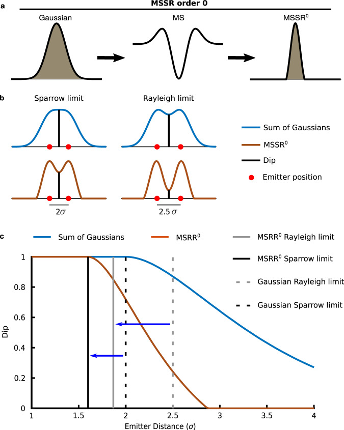
Fig. 1
MSSR of zero order increases resolution by reducing the width of the spatial distribution of photons from simulated fluorescent emitters.
a The MS is applied to the initial Gaussian distribution of photons emitted by a pointu00a0source (left) resulting in a MS graph (center). Application of further algebraic transformations (see Supplem...
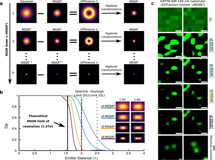
Fig. 2
Single-frame MSSR analysis of higher order attains a resolution limit of 1.6 u03c3 for nearby emitters.
a Higher-order MSSR algorithm (MSSR n ). The first iteration of MSSR (MSSR 1 ) is given by subtracting the MSSR 0 from the original image, resulting in a doughnut-like region centered at the emitteru2...
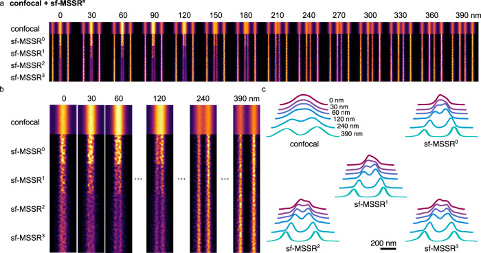
Fig. 3
sf-MSSR n extends spatial resolution in confocal microscopy.
a Comparison of confocal and sf-MSSR n reconstruction ( n =u20090u20133), applied to a spaced fluorescent line pattern. Central lines are gradually being separated by steps ofu00a030u2009nm (0u2009nm,...
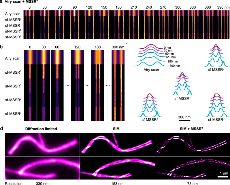
Fig. 4
sf-MSSR n enhances the resolution and contrast of Airyscan and SIM reconstructions.
a Comparison of confocal and sf-MSSR n reconstruction ( n =u20090u20133), applied to a spaced fluorescent line pattern. Central lines are gradually being separated by steps ofu00a030u2009nm (0u2009nm,...
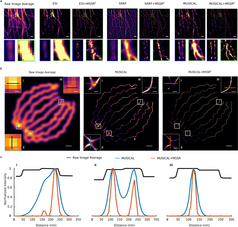
Fig. 5
MSSR furtheru00a0enhancesu00a0the resolution and contrast of SIM or previously super-resolved images.
a Comparison of SRM results of ESI, SRRF and MUSICAL alone and after post-processing with MSSR 0 (ESI + sf-MSSR 0 , SRRF + sf-MSSR 0 , MUSICAL + sf-MSSR 0 ), over a temporal stack of 500 DL images of ...
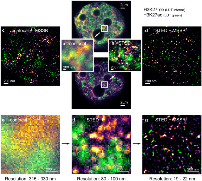
Fig. 6
sf-MSSR n enhances spatial resolution in STED microscopyu00a0images.
a Confocal and b STED micrographs of fluorescent histone protein H3K27 in its acetylated (H3K27ac, i.e., u2018activeu2019, LUT = inferno) or methylated (H3K27me, i.e., u2018inactiveu2019, LUT = green)...
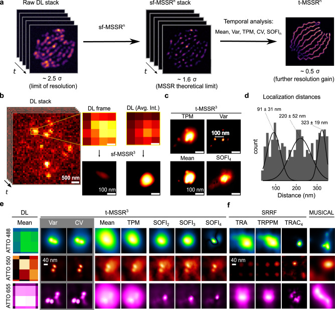
Fig. 7
The temporal analysis of MSSR provides a further increase in resolution to 40u2009nm.
a Single-frame analysis of MSSR of a given order n is applied to each frame of a sequence, becoming the sf-MSSR n stack. Next, a pixel-wise temporal function (PTF) converts the MSSR stack into a singl...
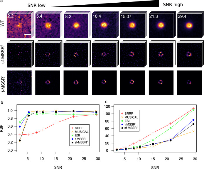
Fig. 8
MSSR is robust to image noise and shows high global performance when compared to other SRM analytical procedures.
a sf-MSSR 1 and t-MSSR 1 of 100 images provide consistent reconstructions across a wide range of SNR. The expected feature is a uniform fluorescent ring located at the center of the image with a dark ...
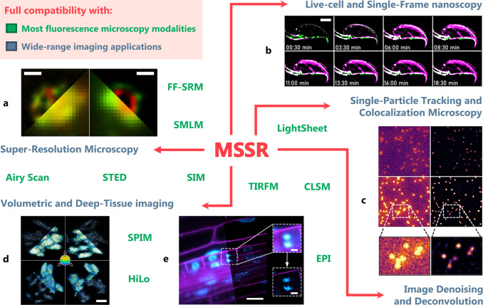
Fig. 9
MSSR applications in fluorescence microscopy.
MSSR operates over images acquired with most fluorescence microscopy modalities available (e.g., widefield, confocal, light-sheet, etc.), denoted by the text in green. It can be applied to achieve enh...
Figure images are served from the NIH/NLM PubMed Central Open Access Subset or Europe PMC; copyright remains with the publishers and authors.
💬 Discussion
0 commentsNo comments yet. Be the first to start a discussion!
Leave a Comment