Abstract
AbstractWe present Richardson–Lucy network (RLN), a fast and lightweight deep learning method for three-dimensional fluorescence microscopy deconvolution. RLN combines the traditional Richardson–Lucy iteration with a fully convolutional network structure, establishing a connection to the image formation process and thereby improving network performance. Containing only roughly 16,000 parameters, RLN enables four- to 50-fold faster processing than purely data-driven networks with many more parameters. By visual and quantitative analysis, we show that RLN provides better deconvolution, better generalizability and fewer artifacts than other networks, especially along the axial dimension. RLN outperforms classic Richardson–Lucy deconvolution on volumes contaminated with severe out of focus fluorescence or noise and provides four- to sixfold faster reconstructions of large, cleared-tissue datasets than classic multi-view pipelines. We demonstrate RLN’s performance on cells, tissues and embryos imaged with widefield-, light-sheet-, confocal- and super-resolution microscopy.
🔬 Techniques
🔭 Microscopes
🧬 Organisms
💻 Software
✨ Fluorophores
🧪 Sample Preparation
🔬 Cell Lines
🏭 Microscope Brands
🧪 Reagent Suppliers
📷 Detectors
💻 Software Details
💻 Code & Software
Image restoration for fluorescence microscopy
Three-dimensional residual channel attention networks
code of the registration and deconvolution project
💾 Data Repositories
🏛️ Research Organizations (ROR)
Affiliated research institutions:
📋 Methods
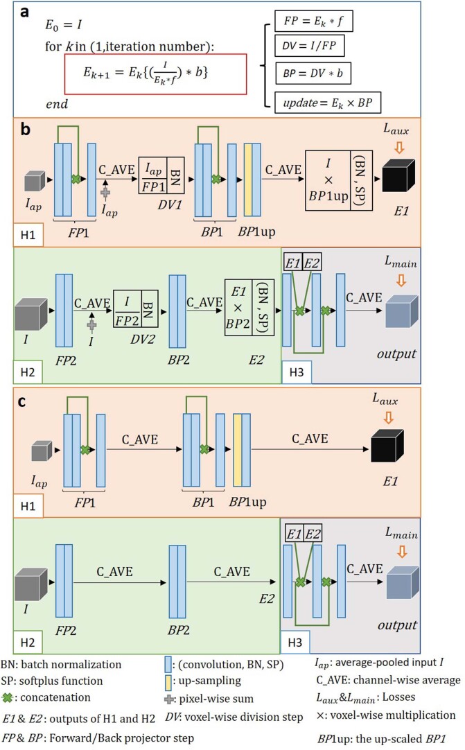
RLN RL deconvolution (equation ( 1 )) has a compact update structure, needing only one formula to update each estimate: 1 documentclass[12pt]{minimal} usepackage{amsmath} usepackage{wasysym} usepackage{amsfonts} usepackage{amssymb} usepackage{amsbsy} usepackage{mathrsfs} usepackage{upgreek} setlength{oddsidemargin}{-69pt} begin{document}$$begin{array}{l}begin{array}{*{20}{l}} {E_0} hfill & = hfill & I hfill \ {{mathrm{for}},k} hfill & = hfill & {0,1, ldots Nleft( {{mathrm{i.e.}},{mathrm{iteration}},{mathrm{number}}} right)} hfill \ {E_{k + 1}} hfill & = hfill & {E_kleft{ {frac{I}{{E_k ast f}} ast b} right}} hfill end{array}\ {mathrm{end}}end{array}$$end{document} E 0 = I for k = 0 , 1 , … N i.e. iteration number E k + 1 = E k I E k * f * b end where * denotes convolution operation, I and E k are the raw input and estimate of the k th iteration and f and b are the forward projector (system PSF) and backward projector, respectively. Traditionally b is taken to be the transpose of f , but using unmatched back projectors (for example, Gaussian, Butterworth or Wiener–Butterworth filters) 8 can result in faster deconvolution by reducing the total number of iterations N needed for achieving a resolution limited result. The key procedure in RLD is convolution. Similarly, convolutional layers are integral to the architecture of deep learning networks, which can learn the convolution kernels automatically. This similarity inspired us to think of using convolutional layers to mimic the convolution with PSF kernels in RL deconvolution. RLN can be regarded as an algorithm unrolling method that uses convolutional layers in a fully convolutional network to represent the convolution steps in each RLD iteration, thereby mimicking the forward/back projection steps. RLN consists of three parts: H1, H2, H3 (Fig. 1a and Extended Data Fig. 1b ). H1 functions similarly to an early iteration in RLD, providing a rough estimate of the final output; H2 acts as a late iteration, using all the information in I to refine the rough estimate and H3 is used to merge and integrate the information provided by H1 and H2. The architecture of H1 and H2 closely follow the RL deconvolution update formula, that is, they mimic the FP and BP steps with convolutional layers, additionally incorporating the division ( DV , documentclass[12pt]{minimal} usepackage{amsmath} usepackage{wasysym} usepackage{amsfonts} usepackage{amssymb} usepackage{amsbsy} usepackage{mathrsfs} usepackage{upgreek} setlength{oddsidemargin}{-69pt} begin{document}$$it frac{I}{{E_k ast f}}$$end{document} I E k * f ), and update steps to learn the correction necessary for improving I . In RLD, FP and BP procedures use relatively large PSF kernels (for example, 128 × 128 × 128 voxels for 0.8 NA/0.8 NA diSPIM). Applying such large kernels in a neural network would degrade training efficiency. Typically, deep learning networks use small convolutional kernels with several convolutional layers to extract features. For efficient operation, larger convolution kernels can be replaced by several smaller convolution kernels 33 , for example a layer of 5 × 5 convolutions can be replaced by two layers each with 3 × 3 convolutions. To maintain network efficiency, H1 uses smaller feature maps and more layers, while H2 uses larger feature maps and less layers. Because H1 only roughly estimates the ground truth, it starts with an average pooling layer to down-scale the input volume (that is, the normalized microscope acquisition I ) by two in all dimensions to obtain I ap (average-pooled input). Although this step may cause information loss, it has the benefit of increasing the FOV, including more spatial information around each voxel, and decreasing computational cost. Following the RL iteration update process, I ap passes through three convolutional layers to construct the forward projection step. We use dense connections 34 among these convolution layers, that is, the outputs of the first two layers are concatenated along the channel direction to act as the input of the third layer, for efficient use of the feature maps. There is also a residual connection between the output feature maps of the third convolution layer and I ap , and the result of this residual connection is denoted FP1 . This residual connection has two functions: (1) the output of the forward projector FP in RL deconvolution is a blurry copy of the current estimate, which approximates the microscope acquisition, and the residual connection acts similarly adding information learned by the network to the current estimate I ap ; and (2) it avoids the risk of dividing by zero in the following division step, which may introduce instability in training. All channels of the residual connection are merged by a channel-wise average (C_AVE) producing FP1 , and the quotient is computed as DV1 = I ap / FP1 . For the back projection step, RLN uses DV1 as the input to three densely connected convolutional layers to construct BP1 . Because the final feature maps of H1 need to be restored to the original size, BP1 is up-scaled by a combination of an up-sampling layer and a convolutional layer to obtain the up-scaled BP1 ( BP1 up). All channels of BP1 up are merged by a channel-wise average to obtain the correction, which is multiplied with I to obtain the estimate E1 . H2 is constructed similarly to H1. The differences are that in the FP and BP steps, there are only two convolutional layers without dense connections; the input of H2 is the original-scale input I , that is, there is no upscaling procedure and the correction is applied to E1 to compute the second estimate E2 . Since H1 already produces a rough estimate, H2 can use fewer parameters. We thus decreased the number of convolutional layers in H2 to improve memory efficiency. H3 consists of three convolution layers and uses dense connections to merge and fine-tune E1 and E2 . After the channel-wise average of the last layer’s feature map, we obtain the final output O . All convolution layers use [3 × 3 × 3] kernels with [1 × 1 × 1] strides, and are followed with batch normalizations 35 and softplus nonlinear activation functions 36 . The up-sampling consists of transpose convolution operations using [2 × 2 × 2] kernels with [2 × 2 × 2] stride, followed with batch normalizations and softplus. The softplus (SP) activation function is a smooth ‘ReLU’ function that ensures nonnegativity and avoids ‘dead regions’ where the gradient vanishes and parameters never update. For DV1 and DV2 , we add a small constant α = 0.001 in the denominator to prevent division by zero. In the unmatched forward/back projectors design 8 , the choice of forward projector is set to the system PSF while the design of the back projector is more flexible, and should take noise amplification into account. Given that the design of the back projector is more complex, we set the number of output channels of the convolutional layers in the forward projector to four and in the backward projector to eight to place more weight on learning the back projectors. The total number of parameters in the RLN is roughly 16,000. For dual-view input, the dual-view information is registered with the ImageJ plugin diSPIM Fusion 8 . RLN merges these registered views by averaging before applying H1 (Supplementary Fig. 6 ). To verify the effectiveness of the DV steps and update steps in RLN, we constructed an ablated version of RLN, named RLN-a (Extended Data Fig. 1c ). RLN-a has the same convolutional layer design as the RLN but removes the DV and update steps. It shares the same loss function and training parameters as RLN. In the training procedure, the loss function is given by: 2 documentclass[12pt]{minimal} usepackage{amsmath} usepackage{wasysym} usepackage{amsfonts} usepackage{amssymb} usepackage{amsbsy} usepackage{mathrsfs} usepackage{upgreek} setlength{oddsidemargin}{-69pt} begin{document}$$L_{{mathrm{total}}} = L_{{mathrm{aux}}} + L_{{mathrm{main}}}$$end{document} L total = L aux + L main where L aux is an auxiliary loss term used to guide H1 training, and L main is the main loss term used to guide training of the whole network. As E1 is the rough estimate of the ground truth, it is expected to be sharper than the input volume I but blurrier than the ground truth GT. Thus, we define intermediate ITM as 3 documentclass[12pt]{minimal} usepackage{amsmath} usepackage{wasysym} usepackage{amsfonts} usepackage{amssymb} usepackage{amsbsy} usepackage{mathrsfs} usepackage{upgreek} setlength{oddsidemargin}{-69pt} begin{document}$${mathrm{ITM}} = 0.8times {mathrm{GT}} + 0.2 times I$$end{document} ITM = 0.8 × GT + 0.2 × I The ratio 0.8 versus 0.2 was empirically chosen, but we found that network output is only weakly dependent on this choice (for example, 0.9 versus 0.1 and 0.7 versus 0.3 work well also and are slightly better than 1.0 versus 0.0). L aux can be computed as the mean square error (m.s.e.) between E1 and ITM: 4 documentclass[12pt]{minimal} usepackage{amsmath} usepackage{wasysym} usepackage{amsfonts} usepackage{amssymb} usepackage{amsbsy} usepackage{mathrsfs} usepackage{upgreek} setlength{oddsidemargin}{-69pt} begin{document}$$L_{{mathrm{aux}}} = {mathrm{m.s.e.}}left( {{mathrm{E}}1,{mathrm{ITM}}} right) = frac{1}{{whd}}mathop {sum}limits_{k = 1}^d {mathop {sum}limits_{j = 1}^w {mathop {sum}limits_{i = 1}^h {left( {{mathrm{E}}1left( {i,j,k} right) - {mathrm{ITM}}left( {i,j,k} right)} right)^2} } } ,$$end{document} L aux = m.s.e. E 1 , ITM = 1 w h d ∑ k = 1 d ∑ j = 1 w ∑ i = 1 h E 1 i , j , k − ITM i , j , k 2 , where d , w , h represents the depth, width and height of the ground truth, respectively. L main includes two parts: the m.s.e. and SSIM 21 between the network output O and GT: 5 documentclass[12pt]{minimal} usepackage{amsmath} usepackage{wasysym} usepackage{amsfonts} usepackage{amssymb} usepackage{amsbsy} usepackage{mathrsfs} usepackage{upgreek} setlength{oddsidemargin}{-69pt} begin{document}$$L_{{mathrm{main}}} = {mathrm{m.s.e.}}left( {O,{mathrm{GT}}} right) - ln left( {left( {1 + {mathrm{SSIM}}left( {O,{mathrm{GT}}} right)} right)/2} right)$$end{document} L main = m.s.e. O , GT − ln 1 + SSIM O , GT / 2 6 documentclass[12pt]{minimal} usepackage{amsmath} usepackage{wasysym} usepackage{amsfonts} usepackage{amssymb} usepackage{amsbsy} usepackage{mathrsfs} usepackage{upgreek} setlength{oddsidemargin}{-69pt} begin{document}$${mathrm{SSIM}}left( {O,{mathrm{GT}}} right) = frac{{left( {2mu _Omu _{{mathrm{GT}}} + C_1} right)left( {2sigma _{O,{mathrm{GT}}} + C_2} right)}}{{left( {mu _O^2 + mu _{{mathrm{GT}}}^2 + C_1} right)left( {sigma _O^2 + sigma _{{mathrm{GT}}}^2 + C_2} right)}},$$end{document} SSIM O , GT = 2 μ O μ GT + C 1 2 σ O , GT + C 2 μ O 2 + μ GT 2 + C 1 σ O 2 + σ GT 2 + C 2 , where μ GT , μ O are the mean values of the GT and O ; documentclass[12pt]{minimal} usepackage{amsmath} usepackage{wasysym} usepackage{amsfonts} usepackage{amssymb} usepackage{amsbsy} usepackage{mathrsfs} usepackage{upgreek} setlength{oddsidemargin}{-69pt} begin{document}$$sigma _{{mathrm{GT}}}^2$$end{document} σ GT 2 , documentclass[12pt]{minimal} usepackage{amsmath} usepackage{wasysym} usepackage{amsfonts} usepackage{amssymb} usepackage{amsbsy} usepackage{mathrsfs} usepackage{upgreek} setlength{oddsidemargin}{-69pt} begin{document}$$sigma _O^2$$end{document} σ O 2 are the variances of the GT and O ; σ GT, O is the covariance of GT and O ; and C 1 and C 2 are small constants that prevent the denominator from becoming zero (here C 1 = 1 × 10 −4 and C 2 = 9 × 10 −4 ). A higher SSIM value means the network output is more similar to the ground truth. Because the SSIM value is smaller than 1, the documentclass[12pt]{minimal} usepackage{amsmath} usepackage{wasysym} usepackage{amsfonts} usepackage{amssymb} usepackage{amsbsy} usepackage{mathrsfs} usepackage{upgreek} setlength{oddsidemargin}{-69pt} begin{document}$${{{mathrm{ln}}}}left( cdot right)$$end{document} ln ⋅ operation is used to keep the loss positive. The m.s.e. term is similar to L aux , ensuring that the difference between network outputs and ground truth is as small as possible, but using m.s.e. exclusively may lead to blurred output. SSIM is used to preserve the global structural similarity between O and GT. The solver method that is used to guide the parameter update is based on the ‘adaptive moment estimation’ (Adam) algorithm. The learning rate r decays during the training procedure according to: 7 documentclass[12pt]{minimal} usepackage{amsmath} usepackage{wasysym} usepackage{amsfonts} usepackage{amssymb} usepackage{amsbsy} usepackage{mathrsfs} usepackage{upgreek} setlength{oddsidemargin}{-69pt} begin{document}$$r = r_0 times {mathrm{dr}}^{frac{{{mathrm{global}}_{mathrm{step}}}}{{{mathrm{decay}}_{mathrm{step}}}}},$$end{document} r = r 0 × dr global _ step decay _ step , where r 0 is the start learning rate, dr is the decay rate, global_step represents the number of training iterations (updated after each iteration) and decay_step determines the decay period. Gaussian filter kernels are used to initialize the convolutional layers in FP, which contain four output channels. Each channel is a Gaussian filter with standard deviation σ = 0.5, 1, 1.5 and 2, respectively: 8 documentclass[12pt]{minimal} usepackage{amsmath} usepackage{wasysym} usepackage{amsfonts} usepackage{amssymb} usepackage{amsbsy} usepackage{mathrsfs} usepackage{upgreek} setlength{oddsidemargin}{-69pt} begin{document}$$begin{array}{l}{{{mathrm{Gaussian}}}}_{{{mathrm{kernel}}}}left( {i - c_i,j - c_j,k - c_k} right)\ = a times {mathrm{exp}}left( { - frac{{left( {i - c_i} right)^2 + left( {j - c_j} right)^2 + left( {k - c_k} right)^2}}{{2sigma ^2}}} right),end{array}$$end{document} Gaussian _ kernel i − c i , j − c j , k − c k = a × exp − i − c i 2 + j − c j 2 + k − c k 2 2 σ 2 , where ( c i , c j , c k ) is the center coordinate of the kernel and a is a random number to increase randomness (ranges from 0.5 to 1). Other kernels in the convolutional layers are randomly initialized with a Gaussian distribution (mean is 0, standard deviation is 1). Using our workstation (see below for details), training with 200 epochs usually takes 2–4 hours, with each epoch using 100 iterations. Real microscopy volumes often exhibit isolated voxels with bright values that represent abnormal structures. Therefore, we adopted the percentile-based normalization as in CARE 9 : 9 documentclass[12pt]{minimal} usepackage{amsmath} usepackage{wasysym} usepackage{amsfonts} usepackage{amssymb} usepackage{amsbsy} usepackage{mathrsfs} usepackage{upgreek} setlength{oddsidemargin}{-69pt} begin{document}$$Nleft( {u;p_{{mathrm{low}}},p_{{mathrm{high}}}} right) = frac{{u - {mathrm{percentile}}left( {u,p_{{mathrm{low}}}} right)}}{{{mathrm{percentile}}left( {u,p_{{mathrm{high}}}} right) - {mathrm{percentile}}left( {u,p_{{mathrm{low}}}} right)}},$$end{document} N u ; p low , p high = u − percentile u , p low percentile u , p high − percentile u , p low , where percentile( u , p ) is the p th percentile of all voxel values of data u . For real data, we set documentclass[12pt]{minimal} usepackage{amsmath} usepackage{wasysym} usepackage{amsfonts} usepackage{amssymb} usepackage{amsbsy} usepackage{mathrsfs} usepackage{upgreek} setlength{oddsidemargin}{-69pt} begin{document}$$p_{{mathrm{low}}} in left( {0,1} right)$$end{document} p low ∈ 0 , 1 and documentclass[12pt]{minimal} usepackage{amsmath} usepackage{wasysym} usepackage{amsfonts} usepackage{amssymb} usepackage{amsbsy} usepackage{mathrsfs} usepackage{upgreek} setlength{oddsidemargin}{-69pt} begin{document}$$p_{{{{mathrm{high}}}}} in left( {99.0,100} right)$$end{document} p high ∈ 99.0 , 100 according to the data quality. For simulated data, we set p low = 0 and p high = 100. We adopted similar online data augmentation as used with 3D RCAN 11 , which is a stochastic block selection process. For every training iteration, the batch size is set to four. The parameters of RLN and the size of selected blocks are summarized in Supplementary Table 3 . For the comparison of RLN with RLD, we implemented both conventional RLD (Figs. 1b,f , 4 and 5 , Extended Data Figs. 2 , 5 , 8 and 10 and Supplementary Figs. 2 – 5 , 7 and 8 ) and RLD with an unmatched back projector (Fig. 2e,h and Extended Data Figs. 3b,c and 4g ). Iteration numbers are included in Supplementary Table 3 . RLN comparison with CARE, RCAN and DDN We benchmarked the performance of RLN versus purely data-driven network structures including CARE, RCAN and DDN, which have demonstrated excellent performance in image restoration. The parameters used in training these neural networks are summarized in Supplementary Table 4 . The CARE implementation was downloaded from https://github.com/CSBDeep/CSBDeep and networks trained according to their instructions ( http://csbdeep.bioimagecomputing.com/doc/ ). According to the default settings, the number of resolution levels of the U-net architecture was set to 2, each level in the down-scaling step and the upscaling step had two convolutional layers, the number of convolutional filters for first resolution level was set to 32 and the convolution kernel size was (3 × 3 × 3). The total number of parameters is almost 1 million. During training, the training batch size was set to four. For the studies using RCAN, we used our recently developed 3D RCAN model ( https://github.com/AiviaCommunity/3D-RCAN ), consisting of five residual groups with each residual group containing five residual channel attention blocks. As default, we used only two convolutional layers in each residual channel attention blocks. Since the convolution kernel size is (3 × 3 × 3) and the convolution channel number is mostly set as 32, the total number of parameters is over 1 million. For DDN, we used our published single-input neural network ( https://github.com/eguomin/regDeconProject/tree/master/DeepLearning ) based on three dense blocks. Here we improved the image preprocessing steps by adding online data augmentation and percentile-based normalization. During training, the training batch size was set to four.
Show full methods section
RLN RL deconvolution (equation ( 1 )) has a compact update structure, needing only one formula to update each estimate: 1 documentclass[12pt]{minimal} usepackage{amsmath} usepackage{wasysym} usepackage{amsfonts} usepackage{amssymb} usepackage{amsbsy} usepackage{mathrsfs} usepackage{upgreek} setlength{oddsidemargin}{-69pt} begin{document}$$begin{array}{l}begin{array}{*{20}{l}} {E_0} hfill & = hfill & I hfill \ {{mathrm{for}},k} hfill & = hfill & {0,1, ldots Nleft( {{mathrm{i.e.}},{mathrm{iteration}},{mathrm{number}}} right)} hfill \ {E_{k + 1}} hfill & = hfill & {E_kleft{ {frac{I}{{E_k ast f}} ast b} right}} hfill end{array}\ {mathrm{end}}end{array}$$end{document} E 0 = I for k = 0 , 1 , … N i.e. iteration number E k + 1 = E k I E k * f * b end where * denotes convolution operation, I and E k are the raw input and estimate of the k th iteration and f and b are the forward projector (system PSF) and backward projector, respectively. Traditionally b is taken to be the transpose of f , but using unmatched back projectors (for example, Gaussian, Butterworth or Wiener–Butterworth filters) 8 can result in faster deconvolution by reducing the total number of iterations N needed for achieving a resolution limited result. The key procedure in RLD is convolution. Similarly, convolutional layers are integral to the architecture of deep learning networks, which can learn the convolution kernels automatically. This similarity inspired us to think of using convolutional layers to mimic the convolution with PSF kernels in RL deconvolution. RLN can be regarded as an algorithm unrolling method that uses convolutional layers in a fully convolutional network to represent the convolution steps in each RLD iteration, thereby mimicking the forward/back projection steps. RLN consists of three parts: H1, H2, H3 (Fig. 1a and Extended Data Fig. 1b ). H1 functions similarly to an early iteration in RLD, providing a rough estimate of the final output; H2 acts as a late iteration, using all the information in I to refine the rough estimate and H3 is used to merge and integrate the information provided by H1 and H2. The architecture of H1 and H2 closely follow the RL deconvolution update formula, that is, they mimic the FP and BP steps with convolutional layers, additionally incorporating the division ( DV , documentclass[12pt]{minimal} usepackage{amsmath} usepackage{wasysym} usepackage{amsfonts} usepackage{amssymb} usepackage{amsbsy} usepackage{mathrsfs} usepackage{upgreek} setlength{oddsidemargin}{-69pt} begin{document}$$it frac{I}{{E_k ast f}}$$end{document} I E k * f ), and update steps to learn the correction necessary for improving I . In RLD, FP and BP procedures use relatively large PSF kernels (for example, 128 × 128 × 128 voxels for 0.8 NA/0.8 NA diSPIM). Applying such large kernels in a neural network would degrade training efficiency. Typically, deep learning networks use small convolutional kernels with several convolutional layers to extract features. For efficient operation, larger convolution kernels can be replaced by several smaller convolution kernels 33 , for example a layer of 5 × 5 convolutions can be replaced by two layers each with 3 × 3 convolutions. To maintain network efficiency, H1 uses smaller feature maps and more layers, while H2 uses larger feature maps and less layers. Because H1 only roughly estimates the ground truth, it starts with an average pooling layer to down-scale the input volume (that is, the normalized microscope acquisition I ) by two in all dimensions to obtain I ap (average-pooled input). Although this step may cause information loss, it has the benefit of increasing the FOV, including more spatial information around each voxel, and decreasing computational cost. Following the RL iteration update process, I ap passes through three convolutional layers to construct the forward projection step. We use dense connections 34 among these convolution layers, that is, the outputs of the first two layers are concatenated along the channel direction to act as the input of the third layer, for efficient use of the feature maps. There is also a residual connection between the output feature maps of the third convolution layer and I ap , and the result of this residual connection is denoted FP1 . This residual connection has two functions: (1) the output of the forward projector FP in RL deconvolution is a blurry copy of the current estimate, which approximates the microscope acquisition, and the residual connection acts similarly adding information learned by the network to the current estimate I ap ; and (2) it avoids the risk of dividing by zero in the following division step, which may introduce instability in training. All channels of the residual connection are merged by a channel-wise average (C_AVE) producing FP1 , and the quotient is computed as DV1 = I ap / FP1 . For the back projection step, RLN uses DV1 as the input to three densely connected convolutional layers to construct BP1 . Because the final feature maps of H1 need to be restored to the original size, BP1 is up-scaled by a combination of an up-sampling layer and a convolutional layer to obtain the up-scaled BP1 ( BP1 up). All channels of BP1 up are merged by a channel-wise average to obtain the correction, which is multiplied with I to obtain the estimate E1 . H2 is constructed similarly to H1. The differences are that in the FP and BP steps, there are only two convolutional layers without dense connections; the input of H2 is the original-scale input I , that is, there is no upscaling procedure and the correction is applied to E1 to compute the second estimate E2 . Since H1 already produces a rough estimate, H2 can use fewer parameters. We thus decreased the number of convolutional layers in H2 to improve memory efficiency. H3 consists of three convolution layers and uses dense connections to merge and fine-tune E1 and E2 . After the channel-wise average of the last layer’s feature map, we obtain the final output O . All convolution layers use [3 × 3 × 3] kernels with [1 × 1 × 1] strides, and are followed with batch normalizations 35 and softplus nonlinear activation functions 36 . The up-sampling consists of transpose convolution operations using [2 × 2 × 2] kernels with [2 × 2 × 2] stride, followed with batch normalizations and softplus. The softplus (SP) activation function is a smooth ‘ReLU’ function that ensures nonnegativity and avoids ‘dead regions’ where the gradient vanishes and parameters never update. For DV1 and DV2 , we add a small constant α = 0.001 in the denominator to prevent division by zero. In the unmatched forward/back projectors design 8 , the choice of forward projector is set to the system PSF while the design of the back projector is more flexible, and should take noise amplification into account. Given that the design of the back projector is more complex, we set the number of output channels of the convolutional layers in the forward projector to four and in the backward projector to eight to place more weight on learning the back projectors. The total number of parameters in the RLN is roughly 16,000. For dual-view input, the dual-view information is registered with the ImageJ plugin diSPIM Fusion 8 . RLN merges these registered views by averaging before applying H1 (Supplementary Fig. 6 ). To verify the effectiveness of the DV steps and update steps in RLN, we constructed an ablated version of RLN, named RLN-a (Extended Data Fig. 1c ). RLN-a has the same convolutional layer design as the RLN but removes the DV and update steps. It shares the same loss function and training parameters as RLN. In the training procedure, the loss function is given by: 2 documentclass[12pt]{minimal} usepackage{amsmath} usepackage{wasysym} usepackage{amsfonts} usepackage{amssymb} usepackage{amsbsy} usepackage{mathrsfs} usepackage{upgreek} setlength{oddsidemargin}{-69pt} begin{document}$$L_{{mathrm{total}}} = L_{{mathrm{aux}}} + L_{{mathrm{main}}}$$end{document} L total = L aux + L main where L aux is an auxiliary loss term used to guide H1 training, and L main is the main loss term used to guide training of the whole network. As E1 is the rough estimate of the ground truth, it is expected to be sharper than the input volume I but blurrier than the ground truth GT. Thus, we define intermediate ITM as 3 documentclass[12pt]{minimal} usepackage{amsmath} usepackage{wasysym} usepackage{amsfonts} usepackage{amssymb} usepackage{amsbsy} usepackage{mathrsfs} usepackage{upgreek} setlength{oddsidemargin}{-69pt} begin{document}$${mathrm{ITM}} = 0.8times {mathrm{GT}} + 0.2 times I$$end{document} ITM = 0.8 × GT + 0.2 × I The ratio 0.8 versus 0.2 was empirically chosen, but we found that network output is only weakly dependent on this choice (for example, 0.9 versus 0.1 and 0.7 versus 0.3 work well also and are slightly better than 1.0 versus 0.0). L aux can be computed as the mean square error (m.s.e.) between E1 and ITM: 4 documentclass[12pt]{minimal} usepackage{amsmath} usepackage{wasysym} usepackage{amsfonts} usepackage{amssymb} usepackage{amsbsy} usepackage{mathrsfs} usepackage{upgreek} setlength{oddsidemargin}{-69pt} begin{document}$$L_{{mathrm{aux}}} = {mathrm{m.s.e.}}left( {{mathrm{E}}1,{mathrm{ITM}}} right) = frac{1}{{whd}}mathop {sum}limits_{k = 1}^d {mathop {sum}limits_{j = 1}^w {mathop {sum}limits_{i = 1}^h {left( {{mathrm{E}}1left( {i,j,k} right) - {mathrm{ITM}}left( {i,j,k} right)} right)^2} } } ,$$end{document} L aux = m.s.e. E 1 , ITM = 1 w h d ∑ k = 1 d ∑ j = 1 w ∑ i = 1 h E 1 i , j , k − ITM i , j , k 2 , where d , w , h represents the depth, width and height of the ground truth, respectively. L main includes two parts: the m.s.e. and SSIM 21 between the network output O and GT: 5 documentclass[12pt]{minimal} usepackage{amsmath} usepackage{wasysym} usepackage{amsfonts} usepackage{amssymb} usepackage{amsbsy} usepackage{mathrsfs} usepackage{upgreek} setlength{oddsidemargin}{-69pt} begin{document}$$L_{{mathrm{main}}} = {mathrm{m.s.e.}}left( {O,{mathrm{GT}}} right) - ln left( {left( {1 + {mathrm{SSIM}}left( {O,{mathrm{GT}}} right)} right)/2} right)$$end{document} L main = m.s.e. O , GT − ln 1 + SSIM O , GT / 2 6 documentclass[12pt]{minimal} usepackage{amsmath} usepackage{wasysym} usepackage{amsfonts} usepackage{amssymb} usepackage{amsbsy} usepackage{mathrsfs} usepackage{upgreek} setlength{oddsidemargin}{-69pt} begin{document}$${mathrm{SSIM}}left( {O,{mathrm{GT}}} right) = frac{{left( {2mu _Omu _{{mathrm{GT}}} + C_1} right)left( {2sigma _{O,{mathrm{GT}}} + C_2} right)}}{{left( {mu _O^2 + mu _{{mathrm{GT}}}^2 + C_1} right)left( {sigma _O^2 + sigma _{{mathrm{GT}}}^2 + C_2} right)}},$$end{document} SSIM O , GT = 2 μ O μ GT + C 1 2 σ O , GT + C 2 μ O 2 + μ GT 2 + C 1 σ O 2 + σ GT 2 + C 2 , where μ GT , μ O are the mean values of the GT and O ; documentclass[12pt]{minimal} usepackage{amsmath} usepackage{wasysym} usepackage{amsfonts} usepackage{amssymb} usepackage{amsbsy} usepackage{mathrsfs} usepackage{upgreek} setlength{oddsidemargin}{-69pt} begin{document}$$sigma _{{mathrm{GT}}}^2$$end{document} σ GT 2 , documentclass[12pt]{minimal} usepackage{amsmath} usepackage{wasysym} usepackage{amsfonts} usepackage{amssymb} usepackage{amsbsy} usepackage{mathrsfs} usepackage{upgreek} setlength{oddsidemargin}{-69pt} begin{document}$$sigma _O^2$$end{document} σ O 2 are the variances of the GT and O ; σ GT, O is the covariance of GT and O ; and C 1 and C 2 are small constants that prevent the denominator from becoming zero (here C 1 = 1 × 10 −4 and C 2 = 9 × 10 −4 ). A higher SSIM value means the network output is more similar to the ground truth. Because the SSIM value is smaller than 1, the documentclass[12pt]{minimal} usepackage{amsmath} usepackage{wasysym} usepackage{amsfonts} usepackage{amssymb} usepackage{amsbsy} usepackage{mathrsfs} usepackage{upgreek} setlength{oddsidemargin}{-69pt} begin{document}$${{{mathrm{ln}}}}left( cdot right)$$end{document} ln ⋅ operation is used to keep the loss positive. The m.s.e. term is similar to L aux , ensuring that the difference between network outputs and ground truth is as small as possible, but using m.s.e. exclusively may lead to blurred output. SSIM is used to preserve the global structural similarity between O and GT. The solver method that is used to guide the parameter update is based on the ‘adaptive moment estimation’ (Adam) algorithm. The learning rate r decays during the training procedure according to: 7 documentclass[12pt]{minimal} usepackage{amsmath} usepackage{wasysym} usepackage{amsfonts} usepackage{amssymb} usepackage{amsbsy} usepackage{mathrsfs} usepackage{upgreek} setlength{oddsidemargin}{-69pt} begin{document}$$r = r_0 times {mathrm{dr}}^{frac{{{mathrm{global}}_{mathrm{step}}}}{{{mathrm{decay}}_{mathrm{step}}}}},$$end{document} r = r 0 × dr global _ step decay _ step , where r 0 is the start learning rate, dr is the decay rate, global_step represents the number of training iterations (updated after each iteration) and decay_step determines the decay period. Gaussian filter kernels are used to initialize the convolutional layers in FP, which contain four output channels. Each channel is a Gaussian filter with standard deviation σ = 0.5, 1, 1.5 and 2, respectively: 8 documentclass[12pt]{minimal} usepackage{amsmath} usepackage{wasysym} usepackage{amsfonts} usepackage{amssymb} usepackage{amsbsy} usepackage{mathrsfs} usepackage{upgreek} setlength{oddsidemargin}{-69pt} begin{document}$$begin{array}{l}{{{mathrm{Gaussian}}}}_{{{mathrm{kernel}}}}left( {i - c_i,j - c_j,k - c_k} right)\ = a times {mathrm{exp}}left( { - frac{{left( {i - c_i} right)^2 + left( {j - c_j} right)^2 + left( {k - c_k} right)^2}}{{2sigma ^2}}} right),end{array}$$end{document} Gaussian _ kernel i − c i , j − c j , k − c k = a × exp − i − c i 2 + j − c j 2 + k − c k 2 2 σ 2 , where ( c i , c j , c k ) is the center coordinate of the kernel and a is a random number to increase randomness (ranges from 0.5 to 1). Other kernels in the convolutional layers are randomly initialized with a Gaussian distribution (mean is 0, standard deviation is 1). Using our workstation (see below for details), training with 200 epochs usually takes 2–4 hours, with each epoch using 100 iterations. Real microscopy volumes often exhibit isolated voxels with bright values that represent abnormal structures. Therefore, we adopted the percentile-based normalization as in CARE 9 : 9 documentclass[12pt]{minimal} usepackage{amsmath} usepackage{wasysym} usepackage{amsfonts} usepackage{amssymb} usepackage{amsbsy} usepackage{mathrsfs} usepackage{upgreek} setlength{oddsidemargin}{-69pt} begin{document}$$Nleft( {u;p_{{mathrm{low}}},p_{{mathrm{high}}}} right) = frac{{u - {mathrm{percentile}}left( {u,p_{{mathrm{low}}}} right)}}{{{mathrm{percentile}}left( {u,p_{{mathrm{high}}}} right) - {mathrm{percentile}}left( {u,p_{{mathrm{low}}}} right)}},$$end{document} N u ; p low , p high = u − percentile u , p low percentile u , p high − percentile u , p low , where percentile( u , p ) is the p th percentile of all voxel values of data u . For real data, we set documentclass[12pt]{minimal} usepackage{amsmath} usepackage{wasysym} usepackage{amsfonts} usepackage{amssymb} usepackage{amsbsy} usepackage{mathrsfs} usepackage{upgreek} setlength{oddsidemargin}{-69pt} begin{document}$$p_{{mathrm{low}}} in left( {0,1} right)$$end{document} p low ∈ 0 , 1 and documentclass[12pt]{minimal} usepackage{amsmath} usepackage{wasysym} usepackage{amsfonts} usepackage{amssymb} usepackage{amsbsy} usepackage{mathrsfs} usepackage{upgreek} setlength{oddsidemargin}{-69pt} begin{document}$$p_{{{{mathrm{high}}}}} in left( {99.0,100} right)$$end{document} p high ∈ 99.0 , 100 according to the data quality. For simulated data, we set p low = 0 and p high = 100. We adopted similar online data augmentation as used with 3D RCAN 11 , which is a stochastic block selection process. For every training iteration, the batch size is set to four. The parameters of RLN and the size of selected blocks are summarized in Supplementary Table 3 . For the comparison of RLN with RLD, we implemented both conventional RLD (Figs. 1b,f , 4 and 5 , Extended Data Figs. 2 , 5 , 8 and 10 and Supplementary Figs. 2 – 5 , 7 and 8 ) and RLD with an unmatched back projector (Fig. 2e,h and Extended Data Figs. 3b,c and 4g ). Iteration numbers are included in Supplementary Table 3 . RLN comparison with CARE, RCAN and DDN We benchmarked the performance of RLN versus purely data-driven network structures including CARE, RCAN and DDN, which have demonstrated excellent performance in image restoration. The parameters used in training these neural networks are summarized in Supplementary Table 4 . The CARE implementation was downloaded from https://github.com/CSBDeep/CSBDeep and networks trained according to their instructions ( http://csbdeep.bioimagecomputing.com/doc/ ). According to the default settings, the number of resolution levels of the U-net architecture was set to 2, each level in the down-scaling step and the upscaling step had two convolutional layers, the number of convolutional filters for first resolution level was set to 32 and the convolution kernel size was (3 × 3 × 3). The total number of parameters is almost 1 million. During training, the training batch size was set to four. For the studies using RCAN, we used our recently developed 3D RCAN model ( https://github.com/AiviaCommunity/3D-RCAN ), consisting of five residual groups with each residual group containing five residual channel attention blocks. As default, we used only two convolutional layers in each residual channel attention blocks. Since the convolution kernel size is (3 × 3 × 3) and the convolution channel number is mostly set as 32, the total number of parameters is over 1 million. For DDN, we used our published single-input neural network ( https://github.com/eguomin/regDeconProject/tree/master/DeepLearning ) based on three dense blocks. Here we improved the image preprocessing steps by adding online data augmentation and percentile-based normalization. During training, the training batch size was set to four.
Training and testing
All networks (RLN, CARE, RCAN and DDN) were implemented with the Tensorflow framework v.1.14.0 and Python v.3.6.2 in the Ubuntu v.16.04.4 LTS operating system. Training and testing were performed on a computer workstation equipped with 32 GB of memory, an Intel(R) Core(TM) i7-8700K, 3.70 GHz CPU and two Nvidia GeForce GTX 1080 Ti GPUs, each with 24 GB of memory. With this workstation, the maximum size of the input data that RLN can be applied to is 320 MB in 32-bit format. For input data sizes that exceed this limit (for example, the large cleared-tissue data shown in Fig. 2d,e,g–i ), our Python-based processing code can automatically crop the volume into several subvolumes, feed them into the RLN network, and stitch the predictions back together. In detail, assuming a data with size W × H × D voxels we first set the depth d of the subvolume as: 10 documentclass[12pt]{minimal} usepackage{amsmath} usepackage{wasysym} usepackage{amsfonts} usepackage{amssymb} usepackage{amsbsy} usepackage{mathrsfs} usepackage{upgreek} setlength{oddsidemargin}{-69pt} begin{document}$${{{{d}}}} = {{{mathrm{min}}}}({{{{D}}}},1,600,{{{mathrm{pixels}}}}),$$end{document} d = min ( D , 1 , 600 pixels ) , then calculate the width w and height h of the subvolume as: 11 documentclass[12pt]{minimal} usepackage{amsmath} usepackage{wasysym} usepackage{amsfonts} usepackage{amssymb} usepackage{amsbsy} usepackage{mathrsfs} usepackage{upgreek} setlength{oddsidemargin}{-69pt} begin{document}$${{{{w}}}},{{{{h}}}} = {{{mathrm{floor}}}}left( {{{{mathrm{sqrt}}}}left( {frac{{frac{{320}}{4} times 1024 times 1024}}{{{{{d}}}}}} right)} right)$$end{document} w , h = floor sqrt 320 4 × 1024 × 1024 d We set the overlapping number voxels in neighboring subvolumes as 24 and use the linear_ramp function (NumPy function) to stitch the overlapped regions. This cropping and stitching procedure is the same as that used in 3D RCAN 11 . Since we did not have access to the true object structure when evaluating the performance of RLN, we used a variety of ‘ground truth’, consisting of high SNR dual-view deconvolved light-sheet data (Figs. 1b and 2 and Extended Data Figs. 3 – 5 ), synthetic ground truth (Fig. 1d,e , Extended Data Figs. 2 and 8a and Supplementary Figs. 2 – 5 ), high SNR deconvolved iSIM data (Fig. 3 and Extended Data Figs. 6 , 7 and 8b ), higher contrast confocal data (Fig. 4 ), super-resolution STED microscopy data (Extended Data Fig. 9 ) and super-resolution 3D SIM data (Extended Data Fig. 10 ). Further details (that is, training ground truth, training pair number, testing type) of training and test datasets are summarized in Supplementary Tables 1 and 3 .
Quantitative analysis
For all datasets, we selected several volumes or slices (4–131) to evaluate the SSIM and PSNR on normalized network outputs and ground truths with MATLAB (Mathworks. R2019b), and then computed the mean value and standard deviation of these volumes. Supplementary Table 2 summarizes these values. The SNR of simulated noisy phantoms (represented as noiseless signal S + different levels of noise N a , Extended Data Fig. 8a and Supplementary Fig. 6 ) were computed as: 12 documentclass[12pt]{minimal} usepackage{amsmath} usepackage{wasysym} usepackage{amsfonts} usepackage{amssymb} usepackage{amsbsy} usepackage{mathrsfs} usepackage{upgreek} setlength{oddsidemargin}{-69pt} begin{document}$${{{mathrm{SNR}}}}_{{{{mathrm{simu}}}}} = 10 times mathop {{log }}nolimits_{10} frac{{{mathrm{Var}}(S)}}{{{mathrm{Var}}(N_{mathrm{a}})}}$$end{document} SNR simu = 10 × log 10 Var ( S ) Var ( N a ) documentclass[12pt]{minimal} usepackage{amsmath} usepackage{wasysym} usepackage{amsfonts} usepackage{amssymb} usepackage{amsbsy} usepackage{mathrsfs} usepackage{upgreek} setlength{oddsidemargin}{-69pt} begin{document}$${mathrm{Var}}left( . right)$$end{document} Var . was used to compute the variance of the volumes. The estimation of SNR of iSIM data (Extended Data Fig. 8b–e ) is the same as used in our earlier 3D RCAN work 11 : 13 documentclass[12pt]{minimal} usepackage{amsmath} usepackage{wasysym} usepackage{amsfonts} usepackage{amssymb} usepackage{amsbsy} usepackage{mathrsfs} usepackage{upgreek} setlength{oddsidemargin}{-69pt} begin{document}$${{{mathrm{SNR}}}}_{{{{mathrm{iSIM}}}}} = S_{{mathrm{iSIM}}}/sqrt {S_{{mathrm{iSIM}}} + N_{mathrm{r}}^2} ,$$end{document} SNR iSIM = S iSIM / S iSIM + N r 2 , where S iSIM is the observed, background-corrected signal in photoelectrons (0.46 photoelectrons per digital count) and N r is the read noise (1.3 electrons according to the manufacturer). Lateral and axial resolution estimates for the data shown in Extended Data Fig. 3d were based on decorrelation analysis 27 of subvolume xz maximum-intensity projections (mean and standard deviations derived from 300 subvolumes, each 600 × 600 × 600 voxels), using a sectorial mask to capture spatial frequencies predominantly along the x and z dimensions, respectively.
Sample preparation
Human osteosarcoma (U2OS, ATCC HTB-96), human T lymphocyte (Jurkat E6-1, ATCC TIB-152, gift from L.E. Samelson, NIH) and African green monkey kidney fibroblast-like cell lines (COS-7, commercially provided by Leica Microsystems) were used in this study. For live cell imaging, the U2OS cells were cultured and maintained at 37 °C and 5% CO 2 on a BIO-133 bottomed-well plate 24 for diSPIM imaging (Fig. 2a–c ), on a no. 1.5 coverslip (VWR, 48393-241) for diSPIM imaging (Supplementary Video 1 ) or on glass bottom dishes (Mattek, P35G-1.5-14-C) for iSIM imaging (Fig. 3 and Extended Data Figs. 6 – 8 ), in 1 ml of DMEM medium (Lonza, 12-604F) containing 10% fetal bovine serum. At 40–60% confluency, cells were transfected with 100 µl of 1× PBS containing 2 µl of X-tremeGENE HP DNA Transfection Reagent (Sigma, 6366244001) and 2 µl of plasmid DNA (300–400 ng µl −1 ) and then maintained at 37 °C, 5% CO 2 for 1–2 days before image acquisition. Cell ER was labeled by ERmoxGFP (Addgene, 68072), mitochondria labeled by mEmerald-Tomm20-C-10 (Addgene, 54281), Golgi apparatus labeled by GalT-GFP (plasmid was a gift from the Patterson Laboratory, NIH, NIBIB) and lysosomes labeled by Lamp1-EGFP (plasmid a gift from the Taraska Laboratory, NIH, NHLBI). Coverslips were prepared as previously described 30 . For widefield/confocal fixed cell imaging (Fig. 4a ), U2OS cells were cultured on a glass bottom dish and fixed in 4% paraformaldehyde/PBS mixture at room temperature for 15 min, then permeabilized by 0.1% Triton X-100/PBS solution at room temperature for 2 min. Cells were rinsed three times by 1× PBS and labeled with 1:100 Alexa Fluor 568 Phalloidin (Thermo Fisher Scientific, A12380). For fixed COS-7 cell imaging (Fig. 4b ), the samples (a gift from Leica Microsystem) were immunolabeled with 500 µl of 1:1,000 anti-NUP primary antibody (clone Mab414) and 1:200 goat-antimouse IgG secondary antibody conjugated with STAR635P. For widefield fixed cell imaging (Fig. 5a–c and Supplementary Fig. 7 ), U2OS cells were cultured and fixed as above. Fixed cells were rinsed three times by 1× PBS and labeled with 500 µl of 1:100 anti-alpha tubulin primary antibody (Thermo Fisher Scientific, 322500), 1:200 anti-Tomm20 primary antibody (Abcam, 78547) and 1:100 Alexa Fluor 647 Phalloidin (Thermo Fisher Scientific, A22287) in 1× PBS at room temperature for 1 h. Labeling mixture was washed away in 1× PBS three times for 1 min for each time. Cells were then labeled with 500 µl of 1:500 Alexa-488 conjugated goat-antimouse secondary antibody (Invitrogen, A11011), 1:500 Alexa-568 conjugated goat-antirabbit secondary antibody (Invitrogen, A-110036) and 1 µg ml −1 DAPI (Thermo Fisher Scientific, D1306) in 1× PBS at room temperature for 1 h. After immunolabeling, cells were washed three times (1 min for each time) in 1× PBS. For confocal/STED imaging (Extended Data Fig. 9 ), U2OS cells were cultured and fixed as above. Fixed cells were immunolabeled with 1:200 anti-Tomm20 primary antibody (Abcam, 78547) and 500 µl of 1:500 donkey antirabbit secondary antibody conjugated with Alexa Fluor 594 (Jackson ImmunoResearch, 711-587-003). For 3D SIM imaging of Jurkat T cells expressing EMTB-3XGFP (Extended Data Fig. 10a ), E6-1 Jurkat cells were cultured in RPMI 1640 supplemented with 10% fetal bovine serum and 1% pen-strep antibiotics. For transient transfections, cells were electroporated using the Neon transfection system (Thermo Fisher Scientific). Briefly, 2 × 10 5 cells were resuspended in 10 μl of R-buffer with 0.5–2 μg of EMTB-3XGFP (Addgene plasmid 26741) and exposed to three pulses of 1,325 V amplitude and 10 ms in duration. Cells were imaged 48 h posttransfection. Coverslips attached to eight-well Labtek chambers were incubated in 0.01% w/v poly- l -lysine (Sigma-Aldrich, P4707) for 10 min. Poly- l -lysine was aspirated and the slide left to dry for 1 h at 37 °C. T cell-activating antibody coating was performed by incubation of slides in a 10 μg ml –1 solution of anti-CD3 antibody (Thermo Fisher Scientific, 14-0039-82) for 2 h at 37 °C or overnight at 4 °C. Excess anti-CD3 was removed by washing with L-15 imaging medium immediately before the experiment. For 3D SIM imaging of fixed U2OS cell expressing Lamp1-EGFP (Extended Data Fig. 10b ), cell cultures at roughly 50% confluency were transfected using xTreme gene HP DNA Transfection Reagent (Sigma, 6366236001). The transfection mixture contained 100 ml of 1× PBS, 2 ml of Transfection Reagent and 1 mg plasmid DNA. LAMP1-EGFP plasmid DNA (gift from G. Patterson’s Laboratory) was used to label lysosomes. The mouse brain sample imaged with 0.4/0.4 NA diSPIM (Fig. 2d ) was prepared using the iDISCO+ procedure and published previously 8 . The tissue section was dissected from an 8-week old male mouse with vasopressin receptor 1B Cre X Ai9 provided by the NIMH (T.B. Usdin and S. Young). The sample was fixed by trans-cardiac perfusion with 4% paraformaldehyde, then dehydrated through a methanol series, rehydrated, immunolabeled with an antibody for tdTomato (Rabbit anti-red fluorescent protein, Rockland Antibodies and Assays, 600-401-379) and an Alexa Fluor 555 secondary antibody (Invitrogen, A27039 ). Before imaging with cleared-tissue diSPIM 8 , the tissue slab was dehydrated with a methanol series and dichloromethane before equilibration in dibenzyl ether (Sigma, 108014). For the cleared mouse brain samples (Fig. 2g , Extended Data Fig. 3b,c and Supplementary Video 2 ), fixed adult mouse brain expressing tdTomato in axonal projections from the area of a stereotaxic injection of adeno-associated virus was cleared using SDS and equilibrated in CUBIC-R 37 . Next, 2 mm thick coronal slabs were sectioned and held in a sample chamber custom designed for the CT-diSPIM. The animal rooms were on a 12-h light cycle, a temperature range of 21–23 °C (70–74 °F) and a humidity range of 30–70%. All animal studies were performed in a manner consistent with the recommendations established by the Guide for the Care and Use of Laboratory Animals (NIH), and all animal protocols were approved by the Animal Care and Use Committees in NIMH. Nematode strains included BV24 (( ltIs44 ( pie-1 p-mCherry::PH(PLC1delta1) + unc-119 (+)); zuIs178 (( his -72 1 kb::HIS-72::GFP); unc-119 (+)) V), Extended Data Figs. 4a,b and 5b , Supplementary Video 3 ), od58 ( ltIs38 (pie-1p::GFP::PH(PLC1delta1) + unc-119(+)) , Fig. 1b and Extended Data Figs. 4c–f and 5a ), AQ2953 ljIs131((myo-3p::GCaMP3-SL2-tagRFP-T), Extended Data Fig. 4g ) and DCR6268 (( pttx-3b ::SL2::Pleckstrin homology domain::GFP::unc-54 3′ UTR + pelt-7 ::mCh::NLS:: unc-54 3′ UTR)), Fig. 5d–f and Supplementary Fig. 8 ). All worms were cultivated at 20 °C on nematode growth medium plates seeded with a lawn of Escherichia coli strain OP50. Embryos were dissected from gravid adults, placed on poly- l -lysine-coated coverslips and imaged in M9 buffer, as previously described 38 . Simulation of phantom objects To evaluate the quality and performance of our network, we generated 3D phantom objects consisting of three types of structure in MATLAB (Mathworks, R2019b, with the Imaging Processing Toolbox) for ground truth: dots, solid spheres and ellipsoidal surfaces (Supplementary Fig. 1 ). Each phantom was composed of 100 solid spheres, 100 ellipsoidal surfaces and 400 dots, randomly located in a 128 × 128 × 128 volume. The 100 solid spheres were generated with random intensity (50–850 counts) and random diameter (4–8 voxels). The 100 ellipsoidal surfaces were generated with random intensity (50–850 counts), random diameter along different axes (4–8 voxels) and random thickness (1–2 voxels); the 400 dots were generated with random intensity (50–850 counts) and random extent along each direction (1–3 voxels). The background value was set to a constant at 30 counts. Noiseless input volumes were generated by convolving the ground truth data with different PSFs (Supplementary Fig. 1 ). Five types of PSF were used, including: the system PSF for the 0.8/0.8 NA diSPIM that has threefold larger axial extent compared to its lateral extent 23 for the generalization test on embryo nuclei and membrane data Extended Data Fig. 5 ); the system PSF of iSIM 11 for the generalization test of ER volumes (Fig. 3e and Extended Data Fig. 7d–f ), the system PSFs of the widefield microscope (Leica, LAS X, DM18, ×63/1.40 OIL ultraviolet) for the generalization test of the fixed U2OS cells and fixed COS-7 cells (Fig. 4 ), the system PSFs of the widefield microscope (Olympus, UPLXAPO60XO, ×60, NA of 1.42 oil objective) for the generalization test of the four-color fixed U2OS cells (Fig. 5a–c ), and the system PSF of the widefield microscope (Olympus UPLSAPO60XWPSF, ×100, NA of 1.35 silicon oil lens) for the generalization test of C. elegans embryo expressing ttx-3B-GFP (Fig. 5d–f ). Noisy images were then obtained by adding different levels of Gaussian and Poisson noise. The 3D human brain phantom was downloaded from the Zubal Phantom website 39 ( http://noodle.med.yale.edu/zubal/data.htm , Fig. 1e,f and Supplementary Fig. 3 ). The simulated spherical phantoms ground truths were generated with ImgLib2 (ref. 22 ) and blurred with a 3D Gaussian kernel with standard deviation set to 2 pixels, the maximum radius of the spheres was set at seven pixels and the intensity range to 80–255 (Fig. 1d and Supplementary Figs. 2 and 5 ). Network inputs of these structures (Fig. 1d,e ) and their corresponding training data were blurred with the system PSF of the 0.8/0.8 NA diSPIM.
DiSPIM data acquisition and processing
A fiber-coupled diSPIM 20 with two ×40, 0.8 NA water objectives (Nikon catalog no. MRD07420), resulting in a pixel size of 162.5 nm, was used to image the U2OS cell transfected with mEmerald-Tomm20-C-10 (Fig. 2a and Supplementary Video 1 ), transgenic embryos strain od58 expressing GFP-membrane (Fig. 1b and Extended Data Figs. 4c–f and 5a ) and BV24 expressing GFP-nuclei (Extended Data Figs. 4a,b and 5b and Supplementary Video 3 ). For cellular imaging, 50–200 dual-view volumes (60 planes, 1 µm interplane spacing in each view) were acquired with 3 s intervals; for embryo imaging, dual-view stacks (50 planes at 1 µm spacing per view) were acquired at 1-min intervals for 291 min. Dual-view data were registered and jointly deconvolved with the diSPIM Fusion ImageJ plugin 8 to generate ground truth, using ten iterations for joint deconvolution.
DiSPIM cleared-tissue acquisition and processing
Cleared-tissue image data in Fig. 2d was acquired on a fiber-coupled diSPIM that was modified for cleared-tissue imaging by incorporating elements of the commercially available ASI DISPIM and DISPIM for Cleared Tissue (CT-DISPIM) 8 . We used a pair of Special Optics 0.4-NA multi-immersion objectives (ASI, 54-10-12). The cleared mouse brain volumes were acquired by moving the stage (2 µm step size, total 4,800 frames with 2,048 × 2,048 pixels) in a raster pattern with the aid of the ASI diSPIM Micromanager plugin ( http://dispim.org/software/micro-manager ). Image data for Fig. 2g were acquired on a dedicated, commercial ASI CT-DISPIM equipped with a pair of Special Optics 0.7-NA multi-immersion objectives (ASI, 54-12-8). Using the DISPIM plugin in Micromanager, we set up a multi-position acquisition in light-sheet mode with unidirectional stage scan. Image FOV was set to 1,536 × 1,536 pixels to avoid geometric distortions near the edge of the full FOV (2,048 × 2,048). Five y positions and two z positions were acquired with 15% overlap, each position was a stack of 1,573 images with a stage step of 1.414 µm. Dual-view data were registered and jointly deconvolved based on Wiener–Butterworth filter back projector (one iteration) for the ground truth, using MATLAB (Mathworks, R2019b, with the Imaging Processing and Parallel Computation Toolboxes) 8 on a computer workstation equipped with Intel(R) Xeon(R) W-2145 CPU at 3.70 GHz and Nvidia Quadro P6000 with 24 GB memory. For joint deconvolution of cleared mouse brain samples in Fig. 2g , running on NIH Biowulf cluster, we modified the code to meet the high-performance computing at NIH requirements for job scheduling. The 28-core ‘gpu’ queue for Biowulf (28 × 2.4 GHz Intel E5-2680v4 processor, four NVIDIA P100 GPUs, 16 GB VRAM, 3,584 cores) was used for computing. iSIM data acquisition and processing A home-built iSIM system 29 with a ×60, 1.2 NA water objective (Olympus UPLSAPO60XWPSF) and an sCMOS camera (PCO, Edge 5.5), resulting in a pixel size of 55 nm, was used to image the U2OS cells (Fig. 3 and Extended Data Figs. 6 – 8 ). All raw volumes were background subtracted and deconvolved using the RL algorithm with 15 iterations to generate ground truth.
Widefield data acquisition and processing
Widefield fixed U2OS and COS-7 cell images (Fig. 4 ) were acquired with a Leica widefield microscope (LAS X, DM18, ×63/1.40 OIL ultraviolet, 102 nm pixel size) and processed with the Leica Thunder computational clearing method (commercial deconvolution software designed for deblurring widefield volumes, using the small volume computational clearing method with default settings, Strategy: Adaptive; Thunder Strength: 60; Thunder Regularization 5.05 × 10 6 ), then the same samples were acquired with Leica confocal microscopy (HC PL APO CS2 ×63/1.40 OIL, a pixel size of 102 nm). The same FOV of widefield and confocal data were found manually, then finely registered with an affine transformation 8 . Widefield fixed U2OS images (Fig. 5a–c and Supplementary Fig. 7 ) were acquired by a home-built widefield microscope with a ×60, 1.42 NA oil objective (Olympus, UPLXAPO60XO) and a pixel size of 266 nm. Widefield C . elegans embryos (Fig. 5d–f and Supplementary Fig. 8 ) were acquired with a ×100, 1.35 NA silicon oil lens (Olympus UPLSAPO60XWPSF) and a pixel size of 111 nm.
Reflective diSPIM data acquisition and processing
The geometry of the diSPIM (0.8/0.8 NA) used for reflective imaging has been previously described 28 . Glass coverslips were sputtering a 150-nm-thick aluminum film over their entire surface and then protecting them with a 700-nm-thick layer of SiO2 (Thin Film Coating). During reflective imaging, four views (direct fluorescence and mirror images) were simultaneously collected in stage scanning mode with the same detection optics. The exposure time for each plane was 5 ms. The ground truth consisted of deconvolving the registered input using a spatially varying PSF and the Wiener–Butterworth unmatched back projector 8 with two iterations (Extended Data Fig. 4g ).
Confocal and STED data acquisition and processing
A commercial Leica STED system (HC PL APO CS2 ×100/1.40 OIL) and a Leica confocal microscopy (HC PL APO CS2 ×63/1.40 OIL) were used to acquire the confocal/STED training and testing datasets (Extended Data Fig. 9 ).
3D SIM data acquisition and processing
A home-built 3D SIM system inspired by previous designs 40 – 43 with a ×60, 1.27 NA water objective was used to image fixed Jurkat T cells expressing EMTB-3XGFP that had settled on anti-CD3 coated coverslips (Extended Data Fig. 10a ) and fixed U2OS cells expressing Lamp1-EGFP (Extended Data Fig. 10b ). The raw 15 input images had a pixel size of 82 nm, and were (1) summed to form diffraction-limited widefield images, then interpolated by a factor of two as input data for RLN training and (2) used to generate 3D SIM reconstructions as ground truth, via a generalized Wiener filter 41 with final pixel size of 41 nm. The microscope will be fully described in a forthcoming publication. Reporting summary Further information on research design is available in the Nature Research Reporting Summary linked to this article.
Online content Any methods, additional references, Nature Research reporting summaries, source data, extended data, supplementary information, acknowledgements, peer review information; details of author contributions and competing interests; and statements of data and code availability are available at 10.1038/s41592-022-01652-7.
Supplementary information Supplementary Information Supplementary Notes 1 and 2, Figs. 1–8 and Tables 1–4. Reporting Summary Peer Review File Supplementary Video 1 Timelapse imaging of live U2OS cell transfected with mEmerald-Tomm20, imaged with diSPIM. Lateral (top) and axial (bottom) maximum-intensity projections are shown, comparing raw data (single view) versus RLN predictions. Volumes were acquired with diSPIM every 3 s, 200 time points. See also Fig. 2a–c. Supplementary Video 2 3D rendering of cleared brain tissue slab (roughly 1.4 × 2.3 × 0.5 mm 3 ) expressing tdTomato in axons acquired with 0.7/0.7 NA cleared-tissue diSPIM, comparing raw single view, dual-view joint deconvolution and RLN prediction. The RLN prediction improves image resolution and contrast relative to the raw input. The joint deconvolution output causes artifacts and shows many fewer neurites relative to the raw input and RLN prediction, likely due to failures of registration between the two raw views. See also Fig. 2g–i and Extended Data Fig. 3. Supplementary Video 3 Nuclear imaging (H2B-GFP) in live C. elegans embryos. Timelapse lateral (top) and axial (bottom) maximum-intensity projections, comparing raw single view, dual-view joint deconvolution ground truth, single-input RLN and dual-input RLN. hpf, hours postfertilization. See also Extended Data Fig. 4.
Supplementary information The online version contains supplementary material available at 10.1038/s41592-022-01652-7.
📊 Figures
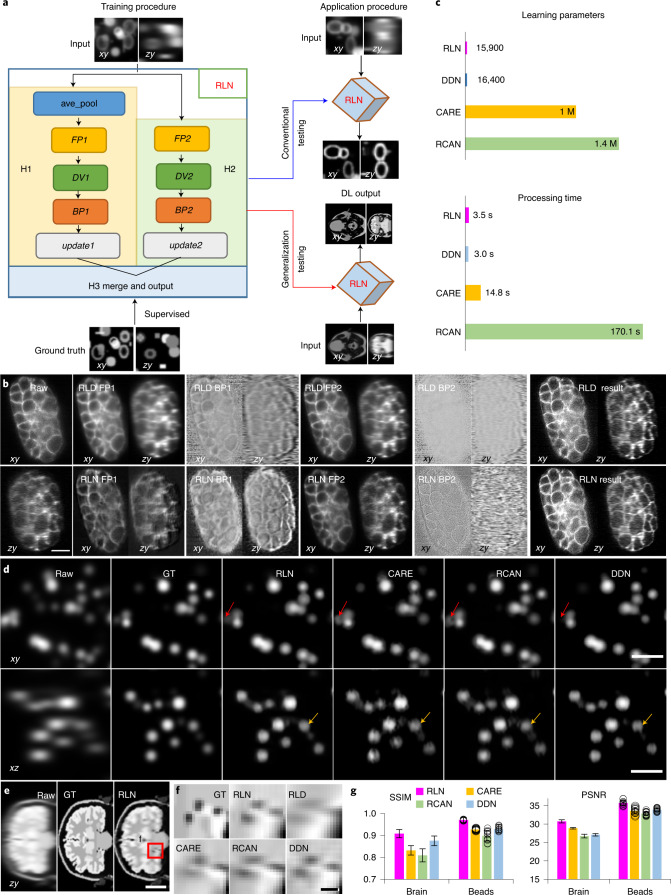
Fig. 1
RLN schematic and performance comparison with CARE, RCAN and DDN.
a , Schematic design of RLN consisting of three parts: H1, H2, and H3. FP1 , DV1 , BP1 , FP2 , DV2 , BP2 in H1/H2 follow the RL deconvolution iterative formula ( Methods ). b , C. elegans embryos expr...
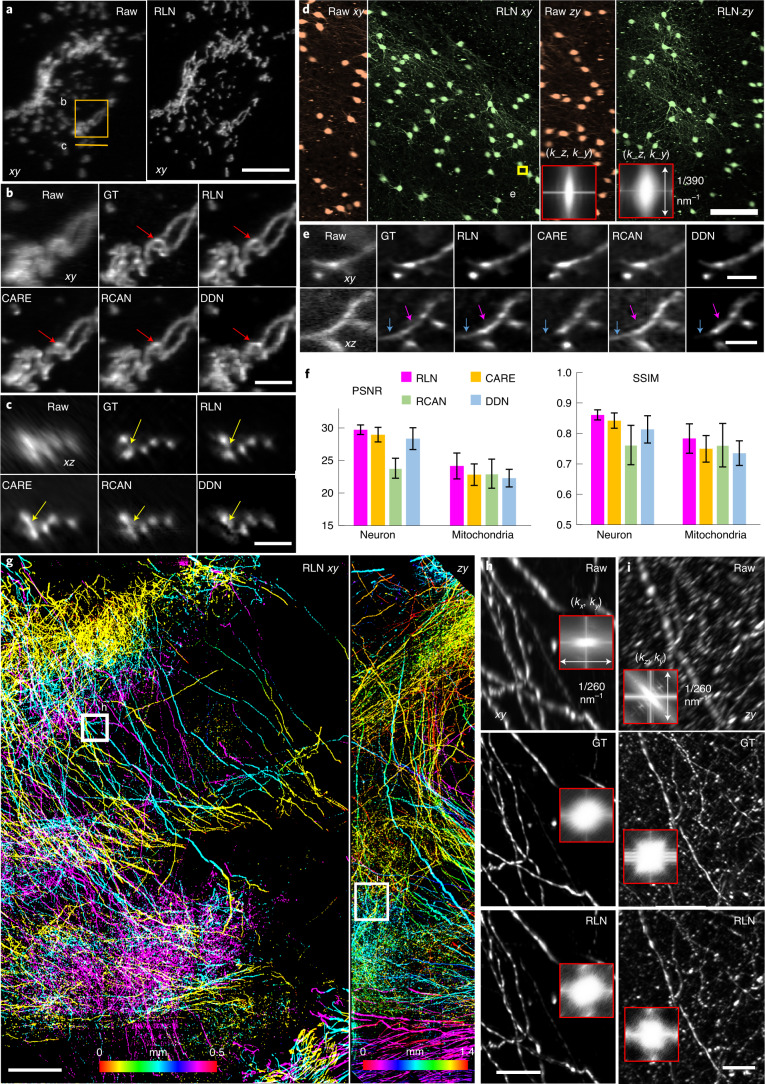
Fig. 2
Deconvolution ability of RLN on thin or cleared biological samples.
a , Live U2OS cells transfected with mEmerald-Tomm20 were imaged with 0.8/0.8 NA diSPIM. Lateral maximum-intensity projections (MIP) of raw single-view and RLN prediction (conventional testing with si...
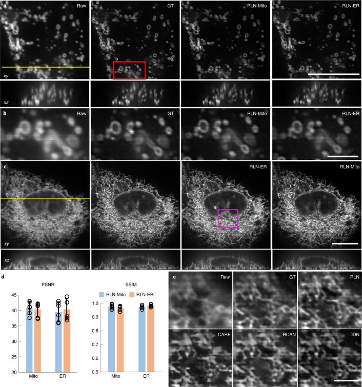
Fig. 3
RLN generalizes well on biological samples.
a , Lateral (top) and axial (bottom) views of live U2OS cells expressing mEmerald-Tomm20-C-10, acquired with iSIM, comparing the raw input (that is, without deconvolution), ground truth (the RL deconv...
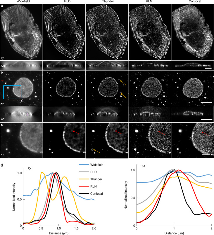
Fig. 4
Comparison between RLN, RLD and Leica Thunder computational clearing method.
a , Lateral and axial planes from images of a fixed U2OS cell stained with Alexa Fluor 568 Phalloidin, comparing widefield raw data, RLD with 100 iterations, Thunder output, RLN result and the registe...
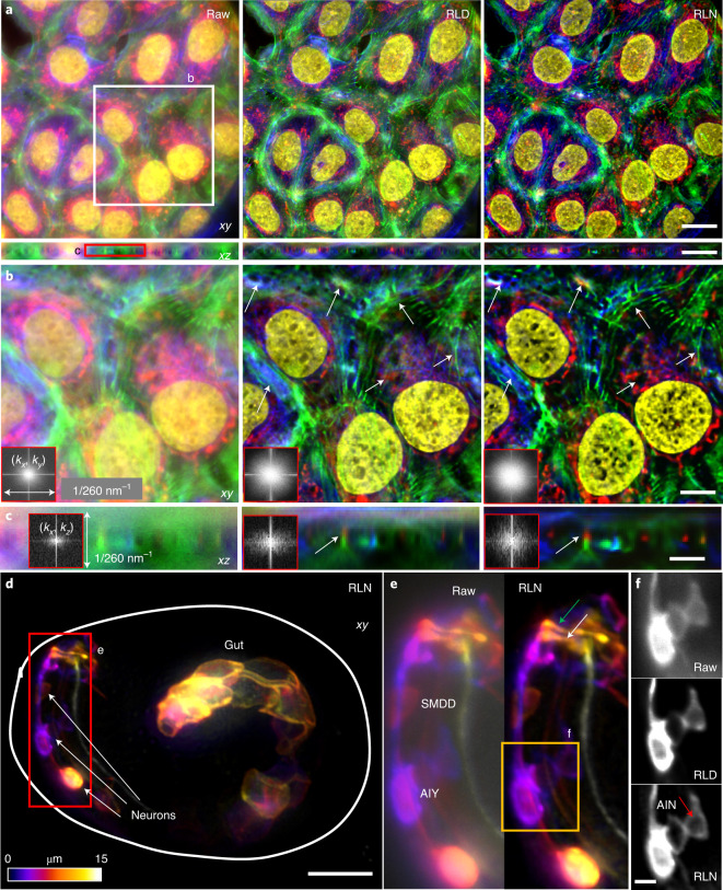
Fig. 5
RLN trained with synthetic mixed structures outperforms direct RLD on volumes contaminated by severe out-of-focus background.
a , Four-color lateral and axial maximum-intensity projections of a fixed U2OS cell, acquired by widefield microscopy, comparing the raw input, RLD and RLN prediction based on a model trained on synth...
Extended Data Fig. 1
Decomposition of RL deconvolution iteration and the internal structure of RLN and RLN-a.
a ) RL deconvolution can be decomposed into four parts: forward projector ( FP ) function, division ( DV ) step, back projector ( BP ) function and update step. b ) Schematic of RLN consisting of thre...
Extended Data Fig. 2
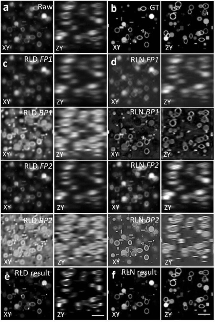
Comparing RLD and RLN on a phantom object consisting of dots, solid spheres, and ellipsoidal surfaces.
Lateral (XY) and axial (ZY) views are presented in each case. a ) Raw input, that is, blurry image. b ) Ground truth object. c ) Intermediate output of RLD. FP1 and BP1 are the forward projector funct...
Extended Data Fig. 3
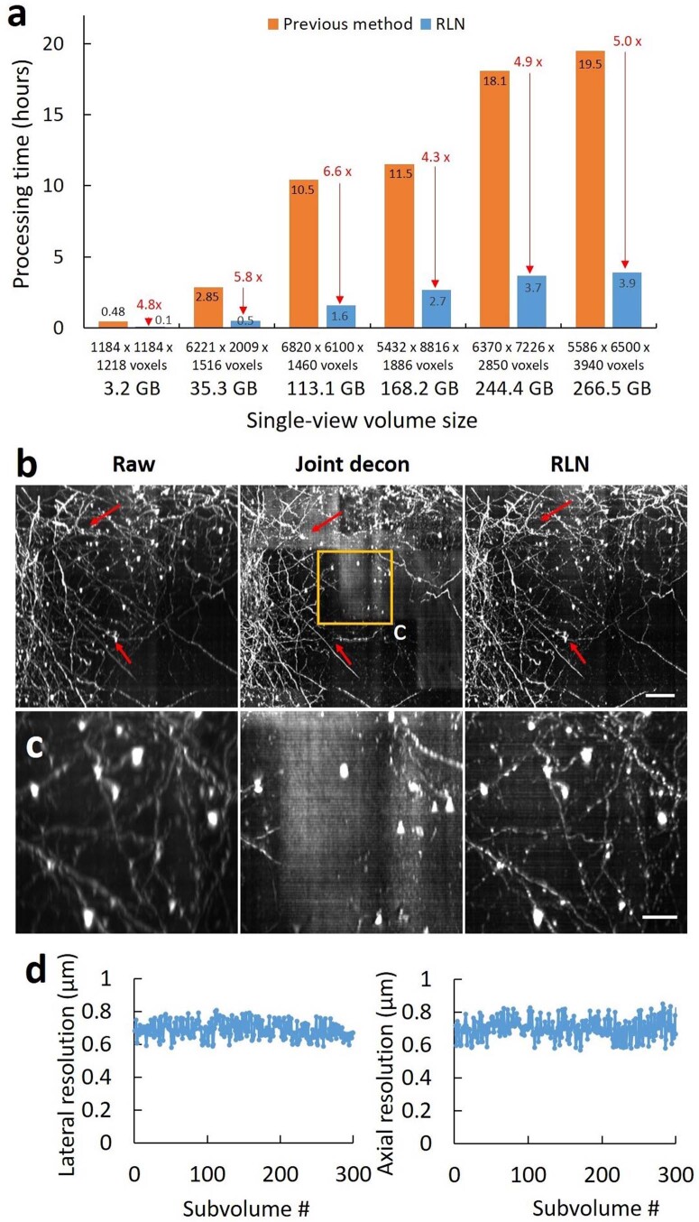
RLN outperforms the previous processing pipeline for reconstructions of large, cleared tissue datasets imaged with diSPIM.
a ) Processing times for RLN vs. previous pipeline on differently sized volumes. In the RLN pipeline, the large raw single-view input volume is cropped into subvolumes, RLN is applied to each subvolum...
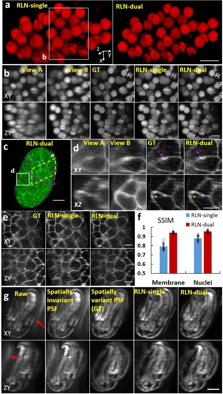
Extended Data Fig. 4
Dual-input RLN improves axial resolution relative to single-input RLN on scattering samples.
a ) 3D rendering of nuclei expressed in live C. elegans embryo collected by diSPIM and processed with single-input RLN and dual-input RLN. b ) Higher magnification of white rectangle in a ), comparing...
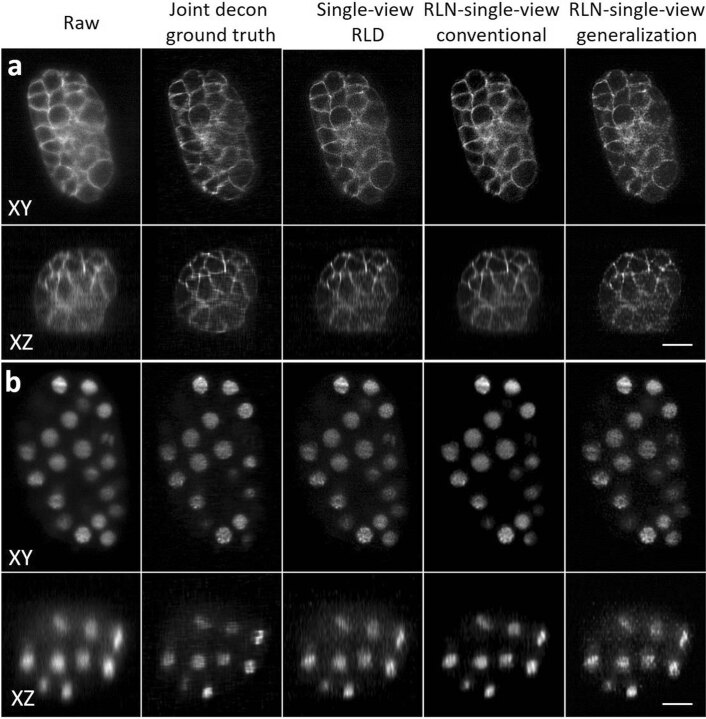
Extended Data Fig. 5
RLN models trained on synthetic mixed data generalize well to images of C. elegans embryos acquired with diSPIM.
a ) Membrane and b ) nuclei results, comparing raw input, dual-view joint deconvolution ground truth, single-view RLD, and predictions from RLN with single-view input under conventional testing (train...
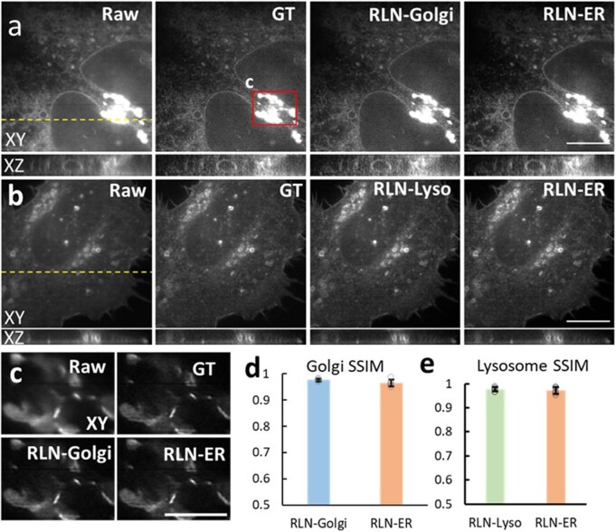
Extended Data Fig. 6
Generalization ability of RLN tested with ER, Golgi, and Lysosome markers, imaged with iSIM.
a ) Lateral and axial views of live U2OS cells expressing GalT-GFP, acquired with iSIM, comparing the raw input, deconvolved iSIM ground truth, predictions from Golgi-trained RLN (RLN-Golgi) and ER-tr...
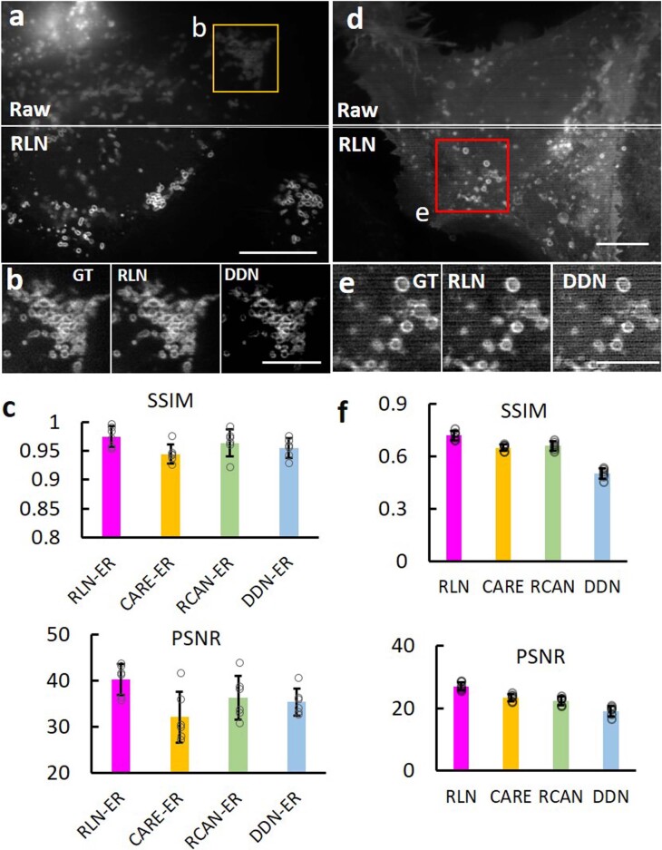
Extended Data Fig. 7
RLN provides better generalization on super-resolution data than other networks.
a ) Super-resolved images of live U2OS cells expressing mEmerald-Tomm20-C-10, acquired with iSIM. Top: raw input; bottom: RLN output. b ) Higher magnification view of yellow rectangular region in a ),...
Extended Data Fig. 8
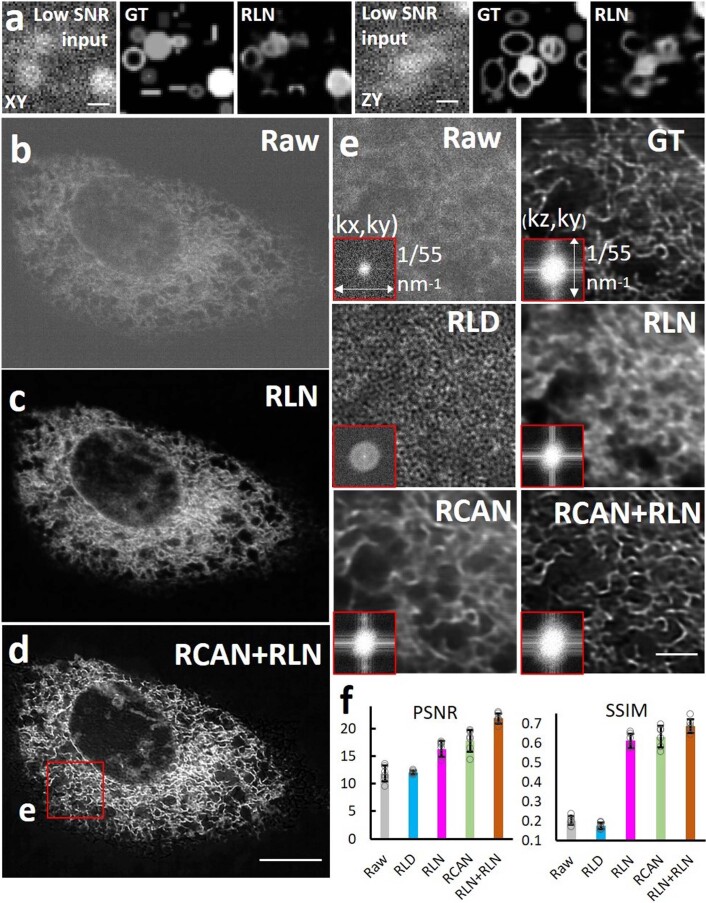
RLNu2019s performance on volumes with very noisy input.
a ) An example of the failure of RLN when challenged with very noisy input. RLN was trained with noisy (SNR 2.45u2009dB) synthetic data (Supplementary Fig. 1 ) and tested on similar structures. Latera...
Extended Data Fig. 9
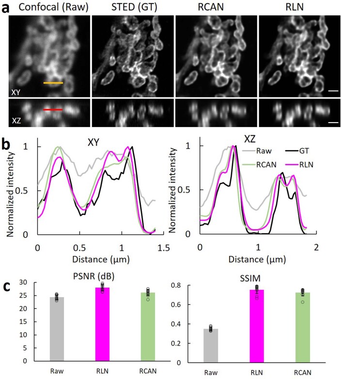
RLN outperforms RCAN when attempting confocal-to-STED cross modality prediction.
a) Lateral views (top) and axial views (bottom) of U2OS cells immunolabeled with a primary antibody against Tomm20 and an anti-rabbit secondary antibody conjugated with Alexa Fluor 594, comparing the ...
Extended Data Fig. 10
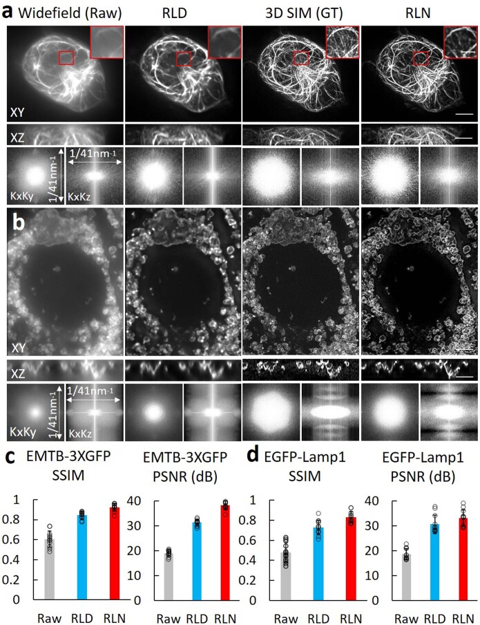
RLN outperforms RLD when attempting to restore widefield data based on 3D SIM ground truth, under both conventional and generalization testing.
a ) Lateral maximum projection (top), axial maximum projection (middle), and Fourier spectra (bottom) of Jurkat cells expressing EMTB-3XGFP, comparing the raw input collected by widefield microscopy, ...
Figure images are served from the NIH/NLM PubMed Central Open Access Subset or Europe PMC; copyright remains with the publishers and authors.
💬 Discussion
0 commentsNo comments yet. Be the first to start a discussion!
Leave a Comment