Abstract
Current super-resolution microscopy (SRM) methods suffer from an intrinsic complexity that might curtail their routine use in cell biology. We describe here random illumination microscopy (RIM) for live-cell imaging at super-resolutions matching that of 3D structured illumination microscopy, in a robust fashion. Based on speckled illumination and statistical image reconstruction, easy to implement and user-friendly, RIM is unaffected by optical aberrations on the excitation side, linear to brightness, and compatible with multicolor live-cell imaging over extended periods of time. We illustrate the potential of RIM on diverse biological applications, from the mobility of proliferating cell nuclear antigen (PCNA) in U2OS cells and kinetochore dynamics in mitotic S. pombe cells to the 3D motion of myosin minifilaments deep inside Drosophila tissues. RIM's inherent simplicity and extended biological applicability, particularly for imaging at increased depths, could help make SRM accessible to biology laboratories.
🔬 Techniques
🔭 Microscopes
🧬 Organisms
💻 Software
✨ Fluorophores
🧪 Sample Preparation
🔬 Cell Lines
🏭 Microscope Brands
🧪 Reagent Suppliers
📷 Detectors
🔎 Objectives
🎨 Filters
💻 Software Details
💾 Data Repositories
🏷️ Research Resource Identifiers (RRIDs)
Verified research resources used in this paper:
🏛️ Research Organizations (ROR)
Affiliated research institutions:
📋 Methods
Key resources table REAGENT or RESOURCE SOURCE IDENTIFIER
Chemicals, peptides, and recombinant proteins Vectashield Vector Laboratories Cat#H-1000 20-hydroxyecdysone Sigma-Aldrich Cat# H5142 DMEM Glutamax + glucose 4.5 g/L, 1 mM sodium pyruvate Invitrogen Cat#10569010 pen/strep Invitrogen Cat#15140148 FCS Eurobio Cat#CVFSVF0601 Geneticin Euromedex Cat#EU0600-A Puromycin Invivogen Cat#ANT-PR-5 Hygromycin Invivogen Cat# ANT-HG-1 EDTA Sigma-Aldrich E5134 RPMI 1640 Invitrogen 21875-034 Macrophage Colony-Stimulating Factor (M-CSF) Peprotech 300-25 SIZE B Alexa Fluor 488-phalloidin Molecular Probes A12379 Alexa Fluor 647-coupled phalloidin Molecular Probes A22287 Mouse anti-vinculin (clone hvin-1) Sigma-Aldrich V9131 Secondary F(ab') 2 coupled to Alexa 555 Cell Signaling Technology 4409 Experimental models: organisms/strains D. melanogaster : Myosin-RFP: w, sqh{TI}-TagRFPt [3B] Ambrosini et al., 2019 CBI, LBCMCP D. melanogaster: Sqh::GFPcrispr Daniel et al., 2018 N/A D. melanogaster: Sqh::UtrABD-GFP, Sqh::RLCmyosinII-mCherry Qin et al., 2017 N/A D. melanogaster : Ecad-GFP: w; shg{TI}-GFP BDSC RRID:BDSC_60584 Streptococcus pneumoniae : strain R3702: FtsZ-GFP Berger et al., 2013 N/A S. pombe : ST102: h - ndc80-GFP:kr cdc11-CFP:kr ura4-D18 leu1-32 ST1771: h + ndc80-GFP:kr cdc11-GFP:kr Tournier et al., 2004 CBI, LBCMCP U2OS cells expressing AsiSI-ER-AID, 53BP1-GFP and mCherry-PCNA Aymard et al. 2014 N/A HUVEC cells: HUV-EC-C (HUVEC) ATCC CRL-1730 C. elegans: Strain wild-type N2 Caenorhabditis Genetics Center RRID: WB-STRAIN N2_(ancestral) Software and algorithms Adobe Illustrator CS5 Adobe RRID:SCR_010279 Fiji https://fiji.sc/ RRID: SCR_002285 ZEN Blue ZEISS RRID:SCR_013672 Black Zen software ZEISS RRID:SCR_018163 Two-colors acquisition software Abbelight and Inscoper N/A One-color acquisition software micromanager N/A AlgoRIM This paper http://cell-rep-meth.rim-microscope.fr Other Schneider’s insect medium Sigma-Aldrich Cat#S0146 Fetal calf serum (FCS) Sigma-Aldrich F7524 Halocarbon oil Sigma-Aldrich Cat#H8773 120 μm deep Secure-Seal™ Sigma-Aldrich Cat#GBL654008 Glass coverslips (0.17 mm ±0.005mm) Marienfeld 0117640 Magnetic microbeads coated with antibodies directed against CD14 Miltenyi Biotec 130-050-20 Resource availability Lead contact Further information and requests for resources and reagents should be directed to and will be fulfilled by the Lead Contact: Thomas Mangeat ( thomas.mangeat@univ-tlse3.fr ).
Show full methods section
Key resources table REAGENT or RESOURCE SOURCE IDENTIFIER
Chemicals, peptides, and recombinant proteins Vectashield Vector Laboratories Cat#H-1000 20-hydroxyecdysone Sigma-Aldrich Cat# H5142 DMEM Glutamax + glucose 4.5 g/L, 1 mM sodium pyruvate Invitrogen Cat#10569010 pen/strep Invitrogen Cat#15140148 FCS Eurobio Cat#CVFSVF0601 Geneticin Euromedex Cat#EU0600-A Puromycin Invivogen Cat#ANT-PR-5 Hygromycin Invivogen Cat# ANT-HG-1 EDTA Sigma-Aldrich E5134 RPMI 1640 Invitrogen 21875-034 Macrophage Colony-Stimulating Factor (M-CSF) Peprotech 300-25 SIZE B Alexa Fluor 488-phalloidin Molecular Probes A12379 Alexa Fluor 647-coupled phalloidin Molecular Probes A22287 Mouse anti-vinculin (clone hvin-1) Sigma-Aldrich V9131 Secondary F(ab') 2 coupled to Alexa 555 Cell Signaling Technology 4409 Experimental models: organisms/strains D. melanogaster : Myosin-RFP: w, sqh{TI}-TagRFPt [3B] Ambrosini et al., 2019 CBI, LBCMCP D. melanogaster: Sqh::GFPcrispr Daniel et al., 2018 N/A D. melanogaster: Sqh::UtrABD-GFP, Sqh::RLCmyosinII-mCherry Qin et al., 2017 N/A D. melanogaster : Ecad-GFP: w; shg{TI}-GFP BDSC RRID:BDSC_60584 Streptococcus pneumoniae : strain R3702: FtsZ-GFP Berger et al., 2013 N/A S. pombe : ST102: h - ndc80-GFP:kr cdc11-CFP:kr ura4-D18 leu1-32 ST1771: h + ndc80-GFP:kr cdc11-GFP:kr Tournier et al., 2004 CBI, LBCMCP U2OS cells expressing AsiSI-ER-AID, 53BP1-GFP and mCherry-PCNA Aymard et al. 2014 N/A HUVEC cells: HUV-EC-C (HUVEC) ATCC CRL-1730 C. elegans: Strain wild-type N2 Caenorhabditis Genetics Center RRID: WB-STRAIN N2_(ancestral) Software and algorithms Adobe Illustrator CS5 Adobe RRID:SCR_010279 Fiji https://fiji.sc/ RRID: SCR_002285 ZEN Blue ZEISS RRID:SCR_013672 Black Zen software ZEISS RRID:SCR_018163 Two-colors acquisition software Abbelight and Inscoper N/A One-color acquisition software micromanager N/A AlgoRIM This paper http://cell-rep-meth.rim-microscope.fr Other Schneider’s insect medium Sigma-Aldrich Cat#S0146 Fetal calf serum (FCS) Sigma-Aldrich F7524 Halocarbon oil Sigma-Aldrich Cat#H8773 120 μm deep Secure-Seal™ Sigma-Aldrich Cat#GBL654008 Glass coverslips (0.17 mm ±0.005mm) Marienfeld 0117640 Magnetic microbeads coated with antibodies directed against CD14 Miltenyi Biotec 130-050-20 Resource availability Lead contact Further information and requests for resources and reagents should be directed to and will be fulfilled by the Lead Contact: Thomas Mangeat ( thomas.mangeat@univ-tlse3.fr ).
Materials availability
This study did not generate new unique reagents.
Data and code availability
The micromanager script monitoring the recording of the speckled raw images in the single-camera RIM implementation and the reconstruction software algoRIM developed for the current study are available at: http://cell-rep-meth.rim-microscope.fr . Speckled raw images are also accessible from the same address, allowing the readers to reproduce some results of the paper.
Experimental models and subject details Podosomes of macrophages
Human monocytes were isolated from blood of healthy donors as described previously ( Van Goethem et al., 2010 ). Cells were re-suspended in cold PBS supplemented with 2 mM EDTA, 0.5% heat-inactivated fetal calf serum (FCS) at pH 7.4 and magnetically sorted with magnetic microbeads coated with antibodies directed against CD14 (Miltenyi Biotec). Monocytes were then seeded on glass coverslips at 1.5x10 6 cells/well in six-well plates in RPMI 1640 (Invitrogen) without FCS. After 2 h at 37°C in humidified 5% CO 2 atmosphere, the medium was replaced by RPMI containing 10% FCS and 20 ng/mL of Macrophage Colony-Stimulating Factor (M-CSF) (Peprotech). For experiments, cells were used after seven days of differentiation. Macrophages plated on glass coverslips (0.17 mm ±0.005mm, Marienfeld) were unroofed and fixed as previously described ( Bouissou et al., 2017 ) and labelled with Alexa Fluor 488-phalloidin (Molecular Probes, 1/500) and Alexa Fluor 647-coupled phalloidin (Molecular Probes, A22287, 1/100) for RIM and dSTORM, respectively. Vinculin was stained using mouse anti-vinculin (clone hvin-1, Sigma-Aldrich, 1/500) and a secondary F(ab') 2 coupled to Alexa 555 (Cell Signaling technology).
Vimentin in HUVEC cells
For immunofluorescence microscopy, HUVEC cells were seeded and grown onto 0.17 mm H coverslip. Cells were fixed with 3.7 % PFA (Sigma Aldrich) in PBS for 10 min at 4°C, and permeabilized with 0.1 % Triton X100 for 10 min at 4°C. After washing thrice with PBS, the cells were incubated for 1h with anti-vimentin rabbit antibody (Sigma Aldrich) and then after washing thrice with PBS, incubated with anti-rabbit Aberrior Star 635P conjugated secondary antibodies (NanoTag Biotechnologies) diluted to 1/10, and subsequently washed three times with PBS for 10 min each. Coverslips were mounted on microscope slides using home-made Mowiol-DABCO. FtsZ ring of S. pneumoniae S. pneumoniae strain containing the FtsZ-GFP fusion (R3702, Bergé et al., 2013), was grown in C+Y medium as previously described at 37°C to an OD 550 of 0.15 ( Bergé et al., 2017 ). Samples were collected, pelleted (3 min, 3,000 g ) and resuspended in cold C medium. The C medium contained per liter: 5 g casein hydrolysate, 6 mg tryptophane, 11.25 mg cysteine, 2 g sodium acetate and 8.5 g K 2 HPO 4 . Cells were spotted on a microscope slide containing a slab of 1.2% agarose in C medium and covered with a pre-treated coverslip before imaging.
PCNA dynamics in U2OS cells
U2OS cells stably expressing AsiSI-ER-AID, 53BP1-GFP and mCherry-PCNA (AID-DivA 53BP1-GFP mCherry-PCNA) ( Caron et al., 2015 ) were cultured in Dulbecco’s modified Eagle’s medium (DMEM Glutamax + glucose 4.5 g/L, 1 mM sodium pyruvate, Invitrogen), antibiotics (pen/strep; Invitrogen), 10% FCS (Invitrogen), 800 μg/mL geneticin (Sigma), 1 μg/mL puromycin (Invivogen), 250 μg/mL hygromycin (Invivogen) at 37°C in a humidified atmosphere with 5% CO2.
Mitosis of S. pombe cells
Media, growth, maintenance of strains, and genetic methods were performed as previously reported ( Moreno et al., 1991 ). Cells were grown at 25°C on yeast extract agar plates. Strain genotype used: ST102 h ndc80-GFP:: kanR cdc11-CFP::kanR ura4-D18 leu1-32. To analyze chromosomes dynamics, kinetochore protein Ndc80 was labeled with a GFP construct (Ndc80-GFP) in wild-type cells. For live-cell analysis, the cells were put on an imaging chamber (CoverWell PCI-2.5; Grace Bio-Labs, Inc.) filled with 1 mL of 1% agarose in minimal medium and sealed with a 22 × 22 mm glass coverslip. To accurately determine the prophase to anaphase A duration in fission yeast, we imaged cells expressing simultaneously Cdc11-GFP (spindle poles) and Ndc80-GFP (kinetochores) (strain ST1771; cdc11-GFP::Kan ndc80-GFP::Kan Leu1-32 Ura4-D18), with RIM or widefield microscopy using the same imaging settings and growth conditions. C. elegans The C. elegans strain used in this study was maintained at 20°C under standard conditions as described in ( Brenner, 1974 ). The ERM-1-GFP strain was FL378:erm-1(bab59[erm-1::mNGˆ3xFlag])I. L4 stages larvae were mounted on a 10% agarose pad in a suspension of 100 nm polystyrene microbeads (Polysciences Inc.) to block worm movements. For transmission electron microscopy (TEM) control L4 larvae were treated as described in ( Bidaud-Meynard et al., 2019 ). Drosophila melanogaster The animal model used here is Drosophila melanogaster , in a context of in vivo / ex vivo experiments. In order to respect ethic principles, animals were anesthetized with CO2 (adults) before any manipulation. To avoid any release of flies outside the laboratory, dead flies were frozen before throwing them. Stocks of living flies were conserved in incubators, either at 18 or 25 degrees to maintain the flies in optimal condition. Fly food contains water, agar (0.8%), sugar (4%), flour (7.4%), yeast (2.8%), moldex (1%) and propionic acid (0.3%). Genotypes and developmental stages are indicated below. Experiments were performed in both males and females indifferently.
Drosophila live and fixed leg samples
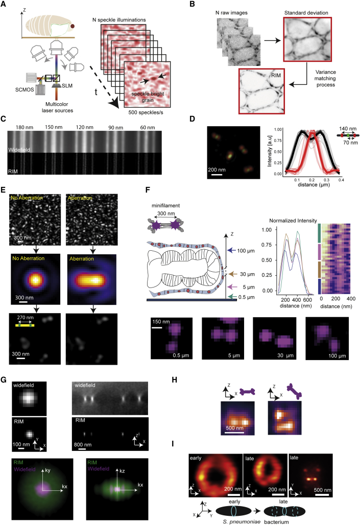
For live imaging, imaginal leg discs from (Sqh-TagRFPt KI [3B]; E-cadherin-GFP) Drosophila strain were freshly dissected from prepupae (2 h after puparium formation) in Schneider medium supplemented with 15% fetal calf serum, 0.5% penicillin-streptomycin and 2 μg/mL 20-hydroxyecdysone (Sigma-Aldrich, H5142) and mounted on slides. For the comparison between Airyscan and RIM and the two-color imaging, imaginal discs were fixed for 20 min in paraformaldehyde (PFA 4%) diluted in PBS. The samples were washed in PBS, re-suspended in Schneider medium and mounted on slides. Drosophila pupa thorax sample Sqh-GFP ( Daniel et al., 2018 ) homozygous or hemizygous Drosophila pupae were maintained at 25°C. Live imaging was performed on pupae aged for 15 to 17h30 APF at 25°C. Pupae were adhered on a glass slide with a double-sided tape, and the brown pupal case was removed over the head and dorsal thorax using microdissecting forceps. Pillars made of 4 and 5 glass coverslips were positioned at the anterior and posterior side of the pupae, respectively. A glass coverslip covered with a thin film of Voltalef 10S oil is then placed on top of the pillars such that a meniscus is formed between the dorsal thorax of the pupae and the glass coverslip ( Gho et al., 1999 ) Drosophila strain for border cells migration Drosophila harboring F-actin labeled by UtrABD-GFP provided by Thomas Lecuit were used to analyze the dynamics of border cells migration. Method details RIM implementation and acquisition parameters The RIM setup is illustrated in Figure S1 A. A Fiber Laser Combiner with 3 fast diode lasers (Oxxius) with respective wavelength 405 nm (LBX-405-180-CSB,) 488 nm (LBX-488-200-CSB), and 561 nm (LMX-561L-200-COL) is used to illuminate the sample. The diode lasers have nanosecond time response for high speed triggering and an Acousto-Optic Modulator is used to modulate the intensity of the solid state 561 nm laser. An apochromatically corrected fiber collimator (RGBV Fiber Collimators 60FC Sukhamburg) produces a collimated TEM 00 2.2 mm diameter output beam for all wavelengths. The incident beam is rotated with an angle of 5 degrees before hitting a X4 Beam Expander beam (GBE04-A) to be shaped into a 8.8 mm TEM 00 beam which illuminates, with the appropriate polarization, a fast Spatial Light binary phase Modulator (SLM : QXGA Fourth Dimensions). The latter is conjugated to the image plane and generates different speckle patterns by displaying masks with randomly independent 0 or π phases at each pixel. Note that the diffuser (here the SLM) could be placed anywhere on the excitation pathway as long as the scattered light filled entirely the pupil at the backfocal plane of the objective. This condition ensured that the frequency cut-off of the speckle pattern at the object plane was 2NA/λ. In practice, the focal lengths of the intermediate lenses were chosen so that, at the back-focal plane of the objective, the extension of the field scattered by the SLM was significantly larger than the pupil. Thus, changing of objective or wavelength did not require any modification of the SLM pattern or lens arrangement because the pupil was always entirely illuminated (at the cost of a variation in the injected power density). The relay lens L1 is an achromatic doublet with visible reflective coating (Thorlabs AC254-500-A). In the intermediate Fourier plane of the illumination path we introduce a quarter wave plate to produce a circular polarization state for the speckled illumination. We also block the zero order of the SLM. A second relay lens system L2 (Thorlabs AC254-150-A) and L3 (Thorlabs AC254-135-A) is used to adapt the beam to all objective lenses. A Quadrichroic Beamsplitter D1 with a cut off centered at 405/488/561/633 nm (Di01-R405/488/561/635-25x36 Semrock) reflects the laser beam towards the inverted microscope (Tei Nikon). The same setup has been used for providing 2D SIM images. In this case, the SLM displays a periodic pattern. At the intermediate Fourier plane of the illumination path, a Fourier mask is introduced to reject the undesired spots from the SLM pixelisation and a pizza laminated polarizer with 12 segments of tangential linear polarization is used to obtain the required linear polarization of the two beams for each azimutal angle (colorPol® VIS 500 BC3 CODIX). Different objective lenses have been used in the experiments and are detailed in Table S1 . Note that, contrary to the SIM mode, changing the objectives or the wavelengths for the RIM mode did not require any change in the SLM masks nor additional tuning. The fluorescence is collected via the objective and tube lens onto one or two (for two-color imaging) SCMOS cameras after appropriate filtering. Three band pass filters (Semrock) were used: FF01-514/30-25 for GFP, FF01-609/54-25 for mCherry and FF01-676/29-25 for the fluorophore used in STED. The 3D image is formed by translating the sample through the focal plane with a piezoelectric Z stage. To synchronize the illumination and data recording, the rolling shutter output of the SCMOS camera is used to trigger the mask change on the SLM. Then, the SLM output triggers the laser when the binary phase mask is stable. A script from micromanager software was written to select the number of speckle patterns per slice, the acquisition time for each speckled image, the number of planes along the Z-axis, the z-spacing and the number of colors used for the acquisition. This script was used for one-color imaging. For two-colors imaging, we used Abbelight and Inscoper softwares. The excitation and emission wavelengths, the characteristics of the objectives, the excitation power density, the number of speckle patterns per slice, the axial excursion and the total acquisition time of all the experiments are given in Tables S1 and S2 of the supplemental information .
Principles of RIM statistical image reconstruction
In this part, we explain how the stack of low-resolution speckled images is processed in order to form one super-resolved reconstruction of the sample. We assume that the object of interest is the thin slice of sample that is located at the focal plane of the microscope. The fluorescence stemming from markers outside the focal plane is considered as noise. The fluorescence density of the sample slice is denoted by f( r ) where r is a two-dimensional vector that indicates a transverse position at the focal plane. The 3D reconstruction is performed by imaging different slices of the sample via a translation through the focal plane. We first summarize the mathematical demonstration of the super-resolution capacity of RIM ( Idier et al., 2018 ) and compare it to that of fluctuation microscopy. Then, we detail the data processing that has been implemented to reach a two-fold resolution gain.
Modeling
RIM data The 2D intensity I of the low-resolution speckled image at the observation point r obs on the camera is a random variable that can be modeled as, (Equation 1) I( r obs )= ∫f( r ) E( r ) H λ’ ( r obs -r ) d r , where f( r ) is the fluorescence density, H λ’ ( r ) is the observation point spread function (PSF) at the fluorescence wavelength λ’ and E( r ) is the speckle intensity. In practice, the speckle pattern is obtained by placing a diffuser on the path of a collimated laser beam of wavelength λ and collecting the scattered light with the microscope objective. Note that in our epi-illumination microscope, the speckle and observation PSF are formed via the same objective of numerical aperture NA. We assume that the speckle is fully developed ( Goodman, 2007 ). In this case, it can be modeled as a sum of plane waves with transverse wave vector k and random phase ϕ( k ) uniformly distributed between 0 and 2π which satisfy, =0 and =δ( k - k ’) where stands for the ensemble average. Note that optical aberrations amount to adding a deterministic phase pattern ψ( k ) to these plane waves. Thus, the probability distribution of ψ(k)+ϕ(k) remains uniformly distributed between 0 and 2π. As a consequence, even though aberrations modify the intensity pattern of a given speckle realization, they do not modify the speckle statistics. The speckle intensity E( r ) at position r can be modeled as, (Equation 2) E( r ) = | ∫p λ ( k ) exp[iϕ( k )] exp[i k.r ] d k | 2 , where p λ ( k )=1 if | k |. Using Equation (2) , one shows that S( r , r’ ) is similar to H λ ( r-r’ ), the point spread function of the microscope at the illumination wavelength λ, defined as, (Equation 4) H λ ( r ) = | ∫l λ ( k ) exp[i k.r ] d k | 2 . The first and second moments of fully developed speckles are thus well known and they are insensitive to scattering distortion or aberration ( Goodman, 2007 ).
Super-resolution capacity of RIM
To eliminate the unknown illuminations from Equation (1) , we form the covariance of the image intensity ( Idier et al., 2018 ), C( r obs1 , r obs2 )=< [I( r obs1 )-] [ I( r obs2 )-] > (Equation 5) = ∫f( r 1 )f( r 2 ) S( r 1 -r 2 ) H λ’ ( r obs1 - r 1 )H λ’ ( r obs2 - r 2 )d r 1 d r 2 which depends on the known speckle covariance and observation PSF. The covariance being a non-negative definite operator, S and C admit unique non-negative definite square roots S 1/2 and C 1/2 which satisfy, ( Mercer, 1909 ) (Equation 6) S( r 1 - r 2 )=∫S 1/2 ( r 1 - r ’) S 1/2 ( r ’- r 2 ) d r ’, where the translational invariance of speckle properties has been used and, (Equation 7) C( r obs1 , r obs2 )=∫C 1/2 ( r obs1 , r ’) C 1/2 ( r ’, r obs2 ) d r ’. Then, the image covariance can be written as, C( r obs1 , r obs2 )=∫C 1/2 ( r obs1 , r ’) C 1/2 ( r ’, r obs2 ) d r ’ (Equation 8) = ∫d r ’ ∫f( r 1 )S 1/2 ( r 1 - r ’) H λ’ ( r obs1 - r 1 ) d r 1 ∫f( r 2 )S 1/2 ( r ’- r 2 ) H λ’ ( r obs2 - r 2 ) d r 2 . Now, if the Fourier support of S is equal or included in that of H λ’, one can filter the speckled images so that the point spread function H λ’ becomes equal to S 1/2 . In this case, the operator K acting on the function q, K(q)= ∫q( r 1 ) S 1/2 ( r 1 - r ’) H λ’ ( r obs1 - r 1 ) d r 1 = ∫ q( r 1 ) S 1/2 ( r 1 - r ’) S 1/2 ( r obs1 - r 1 ) d r 1 is definite and positive so it can be identified to the square root of the image covariance. Then, taking the diagonal terms, one obtains, (Equation 9) C 1/2 ( r , r ) =∫f( r 2 )K( r - r 2 )d r 2 where K( r - r 2 )=S 1/2 ( r - r 2 )S 1/2 ( r - r 2 ). When the speckle is generated through the same objective as the observation point spread function, the Fourier support of S 1/2 is similar to that of H λ’ so the support of K is twice larger than that of H λ’ . Thus, from a theoretical point of view, RIM image covariance bears enough information to reconstruct the fluorescence density with a resolution twice better than that of classical fluorescence microscopy. Note that this demonstration applies identically to three dimensional (3D) imaging by replacing the 2D speckled images, PSF and speckle covariance by 3D ones ( Idier et al., 2018 ).
RIM versus fluctuation microscopy
At this point, one can draw a link between RIM and Fluctuation Microscopy ( Dertinger et al., 2009 ) which is also based on the processing of the second (and sometimes higher) order statistics of ‘random’ images. In fluctuation microscopy, the sample is excited with an homogeneous intensity and one takes advantage of the natural fluctuation (or blinking) of the fluorescence with respect to time to record different realizations of a random imaging process. The images can be modeled using the same Equation 1 as that used for RIM, E being now a random variable accounting for the emission fluctuation. The fundamental difference between speckled illumination and fluctuation microscopy is that, in the first case, the random process exciting the fluorescence is spatially correlated, S=H λ while, in the second case, it is totally uncorrelated and S is a Dirac. This has a major incidence. Trivially, in fluctuation microscopy, the Fourier support of S is not included in that of H λ’ so there is no mathematical proof that the second order statistics of the images can provide the fluorescence density over an enlarged Fourier domain. More precisely, the variance of fluctuation microscopy data simplifiy to a simple convolution of the square of the fluorescence density with the square of the fluorescence density, (Equation 10) V fluctuation ( r ) = C( r,r ) = ∫f 2 ( r 1 )H 2 λ’ ( r - r 1 )d r 1 . This relationship permits to estimate the square of the fluorescence density on the Fourier support of H 2 λ’ . Now, the knowledge of the Fourier transform of f 2 , F (f 2 ), over a domain W, does not imply the knowledge of F (f) over W. Hence, except if f is binary, the super-resolved reconstruction provided by fluctuation microscopy should be taken with caution as it depends on the square of the fluorescence density. In particular, the dynamic range of the fluorophore concentration is generally lost. The weakly and strongly labeled features are often under and over estimated, respectively ( Marsh et al., 2018 ). On the contrary, when the speckle covariance S has a bounded Fourier support, as in RIM, the fluorescence density can theoretically be estimated on an enlarged Fourier support, without loss of the staining dynamic range, as shown in Equation 9 . However, estimating the square root of the speckled image covariance matrix is impossible in practice because of the huge size of the operator. RIM reconstruction algorithm (algoRIM) A tractable technique consists in developing a marginal inversion procedure ( Idier et al., 2018 ) in which the fluorescence density is estimated so as to minimize the distance between the recorded image covariance and the simulated one. Yet, while efficient, this approach cannot be applied to large fields of view as it is computationally demanding, the covariance operator scaling as MxM where M is the number of pixels on the camera. In this work, we propose a simplified approach in which the fluorescence density is estimated so as to minimize the distance between the variance model C( r , r’ ) and the empirical variance. Note that the covariance C( r , r’ ) is maximal at r’ = r and tends towards 0 when r’ moves away from r with a typical decorrelation length corresponding to the width of the observation Point Spread Function (PSF). Thus, most of the information on the fluorescence density is contained about the diagonal of the covariance. Once N different speckled images I l=1...N of the sample have been recorded, the data processing comprises three steps: 1) Each speckled image is deconvolved with a Tikhonov regularised inverse filter. More precisely, we calculate i l so that, (Equation 11) F (i l ) ( k ) = F (I l )( k ) x F (H λ ) ∗ ( k ) / [|F (H λ )( k ) | 2 + e] where e is a parameter (Tikhonov regularization) which depends on the noise level of the raw speckled image, F (g) stands for the Fourier Transform of g and a ∗ is the conjugate of a. The deconvolved image i l can be written as, (Equation 12) i l ( r )= ∫f( r ) E l ( r ) h( r obs - r )d r where we have introduced a novel point spread function, h, such as F (h) ( k ) = |F (H λ )| 2 ( k ) / [|F (H λ )( k ) | 2 + e] The width of this novel PSF being smaller, the information contained by the covariance of the deconvolved speckled images is further concentrated about the diagonal, i.e. the variance. 2) Second, we estimate the empirical variance of i l as (Equation 13) v( r ) =∑ l = 1 … N [i l ( r ) – i ( r ) ] 2 /N, where i ( r ) = ∑ l = 1 … N i l ( r )/N . Third, we estimate f so as to minimize the cost functional, (Equation 14) G(f) = ∫|v( r )-V(f, r )| 2 d r / ∫ |v( r )| 2 d r (Equation 15) where V(f, r ) = C( r , r ) = ∫f( r 1 )f( r 2 ) S( r 1 −r 2 ) h( r - r 1 )h( r - r 2 )d r 1 d r 2 . To minimize G, one needs a solver able to calculate V for a given estimation of the fluorescence f. Now, the calculation of V involves a time consuming quadruple integral, Equation (15) . To speed up the iterative reconstruction procedure, we developed an approximate expression of V which necessitates only a double integral. To this aim, we recall that functions of two variables can be written as a series of the product of functions of one variable only. Let us introduce the bivariate real function, (Equation 16) T( r 1 , r 2 ) = S( r 1 - r 2 ) h(- r 1 )h(- r 2 ). Being a non-negative definite kernel, T admits an eigenvalue decomposition as, (Equation 17) T( r 1 , r 2 ) = ∑ k = 1 … ∞ U k ( r 1 )U k ( r 2 ). In practice, T is discretized over the pixels of the camera and implemented as an Hermitian matrix. Its eigenvalue decomposition yields the eigenvectors of decreasing norm U k . Then, the decomposition is stopped at the K th order, (K about 10 is usually sufficient to have an accurate estimation of T). We thus obtain a limited rank approximation of T. Other limited-rank approximations are possible, but the one we choose reaches an optimal trade-off according to the Eckart–Young theorem ( Eckart and Young, 1936 ). The variance is then calculated using, (Equation 18) V(f, r ) ≈ ∑ k = 1 … K [w k (f, r )] 2 (Equation 19) with w k (f, r ) = ∫f( r 1 )U k ( r 1 − r )d r 1 . It is worth noting that decomposing T( r 1 , r 2 ) is much more efficient than decomposing S( r 1 − r 2 ). Indeed, we have found that the number of eigenvectors required for approximating T is significantly smaller than that required for approximating S with the same accuracy. The minimization of G is performed using a standard conjugate gradient descent algorithm ( Bertero, 1998 ). At each iteration, f( r ) is modified following, f n ( r ) = f n−1 ( r ) + αg n ( r ) where, (Equation 20) g n ( r ) = -2 ∫ [∑ k=1...K w k (f n−1 , r 1 ) U k ( r − r 1 ) ] b( r 1 ) d r 1 with b( r 1 ) = v( r 1 )-V(f n−1 , r 1 ) is the residue and α is the scalar that minimizes the fourth order polynom g(α)= G[ f n−1 + αg n ] (calculated analytically). We use an early-stopping of the iterative process as a simple (but efficient) regularization technique that basically acts as a Tikhonov regularization ( Bertero, 1998 ) to account for the variance noise.
Details on RIM reconstruction procedure
The reconstruction process algoRIM consists in a Tikhonov regularized inverse filter of the raw speckled images, involving the observation PSF, H λ’ , and an iterative estimation of the fluorescence density via the minimization of the distance between the experimental variance of the speckled images and the variance model. The variance matching process involves the speckle covariance H λ .
Estimation of the observation
PSF and accounting for the focal shift phenomenon Ideally, the observation PSF should be estimated from the raw images to account for the possible aberrations on the emission side. This technique was applied in Figure 1 E where the aberrated and non aberrated PSF were estimated from images of 200 nm fluorescent beads using an iterative method which jointly optimizes the PSF (which is assumed to be the same for all the beads) and the beads positions and amplitudes ( Debarnot et al., 2020 ). In all the other experiments, the observation PSF was estimated theoretically. In this case, we paid a particular attention to the aberration induced by the difference between the refractive indices of the oil immersion objective and that of the mounting medium. This aberration widens the PSF and shifts the focal plane as one images deeper in the sample ( Sibarita, 2005 ; Bratton and Shaevitz, 2015 ). To deal with this important issue, we used the PSF models of ( Gibson and Lanni, 1992 ) or ( Khadir et al., 2019 ) which take into account the possible mismatch between the refractive indices of oil, coverslip and mounting medium. First, we estimated the distance D between the coverslip and the theoretical focal plane (which is placed at the working distance specified by the objective). D is equal to 0 when the focal plane coincides with the coverslip surface and increases, as indicated by the Z-stage, when the coverslip is moved away to image deeper in the sample. Then, for a given D, we simulated images of fluorophores at different positions along the z-axis. The image obtained with the highest intensity yielded the two-dimensional PSF. It also indicated the ‘true’ axial position of the observation plane. The latter value was a key parameter when reconstructing the 3D images from successive z-slices and for indicating the depth at which the image was taken. We found the effective position of the observation plane to be 0.66 (for small D ) to 0.87 (for large D ) times smaller than the position indicated by the Z-stage (piezo) ( Sibarita, 2005 ; Bratton and Shaevitz, 2015 ). This correcting factor was included in the 3D image reconstructions and in the depth indications.
Estimation of the speckle covariance
The speckle statistics being insensitive to aberrations, H λ was always estimated theoretically using Equation (4) and adapting the filter I λ to account for the slide-sample transmission coefficient. Tuning parameters of algoRIM All the raw data were interpolated using zero padding to provide pixel sizes at least twice smaller than the Nyquist limit. The observation Point Spread Functions (PSF), H λ , was generated over a grid corresponding to that of the final reconstruction. The number K of eigenvectors used for estimating the variance was always taken equal to 10. The Tikhonov regularized inverse filter parameter used in the deconvolution of the raw images (from 10 −3 to 10 −1 ) and the number of iterations of the variance matching procedure (from 10 to 50) depended on the signal to noise ratio. The computing time per reconstruction varied from 5 s to 140 s on an Intel(R) Xeon(R) CPU E5-2687W v4 at 3.00GHz with 192 RAM, depending on the number of raw speckled images and the number of pixels per image. Artifacts in RIM reconstructions We have shown in ( Idier et al., 2018 ) that, in the limit of an infinite number of speckled illuminations, one could extract, from the covariance of the raw images, the Fourier transform of the true object, within a bounded domain W corresponding to the support of the square of the observation point spread function, Equation 9 . More recently, we have shown in ( Labouesse et al., 2020 ) that there is a one to one correspondence between the variance of the raw images and the Fourier transform of the object over W. Hence, asymptotically, RIM reconstructions are artifact-free within the accessible Fourier domain in the same way as SIM reconstructions when the illumination patterns are perfectly known (and the data noiseless). In practice, if there are enough speckled illuminations for RIM or if the illumination patterns are sufficiently well-known for SIM, there is no bias in the super-resolved image except for the one stemming from a standard zero order Tikhonov regularization introduced to deal with noise. This property distinguishes RIM from other reconstruction methods found in fluctuation or localization microscopy that rely on a priori information on the sample such as binarity, positivity or sparsity and yield biased reconstructions when the samples depart from these assumptions. Yet, in practice, RIM reconstructions are subject to statistical fluctuations because of the limited number N of available raw speckled images. Figure S1 C shows the reconstructions of homogeneous fluorescent lines as a function of N. This study gives an idea of the granule-like artifacts induced by a poor estimation of the speckled image variance. It is shown that for N>400, the granularity contrast is about 10 %. Unfortunately, it seems difficult to estimate a posteriori the level of this artifact as one cannot distinguish the sample spatial fluctuations from the spatial fluctuations induced by a poor estimation of the empirical variance of the raw images. Presently, the best solution for determining the optimal N for a given type of sample is to study the convergence of the reconstruction versus N on one example. Another issue is the noise (photon noise and camera noise) which restricts the domain of spatial frequencies that is accessible for the super-resolved reconstruction. We observed that an important condition for RIM to succeed was that the standard variation of the raw images (obtained with different speckled illuminations) be two and a half times bigger than the standard variation of repeated acquisitions of one particular raw image (with a fixed speckled illumination) (see Figure S1 A for an example of typical raw speckled images). This condition indicates the level of noise (Poisson noise stemming from out-of-focus fluorescence and/or camera electronic noise) that RIM can put up with to provide super-resolved reconstructions.
RIM dynamic imaging
RIM temporal resolution, phototoxicity, and photobleaching depend on the number N of raw speckled images (the stack size) necessary for the homogeneity of the reconstruction ( Figure S1 C), the acquisition time per raw image (limited by the camera) and the excitation intensity (monitoring the noise level, see Figure S1 A). We observed that RIM required the same global photon budget as SIM for the reconstruction process to be successful ( Figures 2 A and 2C). Thus, the high number of 50-200 raw image acquisitions per plane in RIM (compared to 9 or 15 raw images per plane in 2D/3D SIM) could be compensated by a smaller acquisition time per raw image (2-12ms) and a low excitation intensity (4-20 W/cm 2 ) to provide temporal resolution, phototoxicity and photobleaching levels compatible with many live-cell imaging applications. In practice, to image a dynamic process using RIM, raw speckled images were recorded regularly with the smallest possible acquisition time allowed by the camera. The stack size N was determined a posteriori by searching the best trade-off between motion blur and reconstruction noise (using comparisons with similar fixed samples). Then, the super-resolved movie frames were formed using either successive stacks of N raw images (sequential approach) or overlapping stacks of N raw images shifted every P images with P (Equation 5) = ∫f( r 1 )f( r 2 ) S( r 1 -r 2 ) H λ’ ( r obs1 - r 1 )H λ’ ( r obs2 - r 2 )d r 1 d r 2 which depends on the known speckle covariance and observation PSF. The covariance being a non-negative definite operator, S and C admit unique non-negative definite square roots S 1/2 and C 1/2 which satisfy, ( Mercer, 1909 ) (Equation 6) S( r 1 - r 2 )=∫S 1/2 ( r 1 - r ’) S 1/2 ( r ’- r 2 ) d r ’, where the translational invariance of speckle properties has been used and, (Equation 7) C( r obs1 , r obs2 )=∫C 1/2 ( r obs1 , r ’) C 1/2 ( r ’, r obs2 ) d r ’. Then, the image covariance can be written as, C( r obs1 , r obs2 )=∫C 1/2 ( r obs1 , r ’) C 1/2 ( r ’, r obs2 ) d r ’ (Equation 8) = ∫d r ’ ∫f( r 1 )S 1/2 ( r 1 - r ’) H λ’ ( r obs1 - r 1 ) d r 1 ∫f( r 2 )S 1/2 ( r ’- r 2 ) H λ’ ( r obs2 - r 2 ) d r 2 . Now, if the Fourier support of S is equal or included in that of H λ’, one can filter the speckled images so that the point spread function H λ’ becomes equal to S 1/2 . In this case, the operator K acting on the function q, K(q)= ∫q( r 1 ) S 1/2 ( r 1 - r ’) H λ’ ( r obs1 - r 1 ) d r 1 = ∫ q( r 1 ) S 1/2 ( r 1 - r ’) S 1/2 ( r obs1 - r 1 ) d r 1 is definite and positive so it can be identified to the square root of the image covariance. Then, taking the diagonal terms, one obtains, (Equation 9) C 1/2 ( r , r ) =∫f( r 2 )K( r - r 2 )d r 2 where K( r - r 2 )=S 1/2 ( r - r 2 )S 1/2 ( r - r 2 ). When the speckle is generated through the same objective as the observation point spread function, the Fourier support of S 1/2 is similar to that of H λ’ so the support of K is twice larger than that of H λ’ . Thus, from a theoretical point of view, RIM image covariance bears enough information to reconstruct the fluorescence density with a resolution twice better than that of classical fluorescence microscopy. Note that this demonstration applies identically to three dimensional (3D) imaging by replacing the 2D speckled images, PSF and speckle covariance by 3D ones ( Idier et al., 2018 ).
RIM versus fluctuation microscopy
At this point, one can draw a link between RIM and Fluctuation Microscopy ( Dertinger et al., 2009 ) which is also based on the processing of the second (and sometimes higher) order statistics of ‘random’ images. In fluctuation microscopy, the sample is excited with an homogeneous intensity and one takes advantage of the natural fluctuation (or blinking) of the fluorescence with respect to time to record different realizations of a random imaging process. The images can be modeled using the same Equation 1 as that used for RIM, E being now a random variable accounting for the emission fluctuation. The fundamental difference between speckled illumination and fluctuation microscopy is that, in the first case, the random process exciting the fluorescence is spatially correlated, S=H λ while, in the second case, it is totally uncorrelated and S is a Dirac. This has a major incidence. Trivially, in fluctuation microscopy, the Fourier support of S is not included in that of H λ’ so there is no mathematical proof that the second order statistics of the images can provide the fluorescence density over an enlarged Fourier domain. More precisely, the variance of fluctuation microscopy data simplifiy to a simple convolution of the square of the fluorescence density with the square of the fluorescence density, (Equation 10) V fluctuation ( r ) = C( r,r ) = ∫f 2 ( r 1 )H 2 λ’ ( r - r 1 )d r 1 . This relationship permits to estimate the square of the fluorescence density on the Fourier support of H 2 λ’ . Now, the knowledge of the Fourier transform of f 2 , F (f 2 ), over a domain W, does not imply the knowledge of F (f) over W. Hence, except if f is binary, the super-resolved reconstruction provided by fluctuation microscopy should be taken with caution as it depends on the square of the fluorescence density. In particular, the dynamic range of the fluorophore concentration is generally lost. The weakly and strongly labeled features are often under and over estimated, respectively ( Marsh et al., 2018 ). On the contrary, when the speckle covariance S has a bounded Fourier support, as in RIM, the fluorescence density can theoretically be estimated on an enlarged Fourier support, without loss of the staining dynamic range, as shown in Equation 9 . However, estimating the square root of the speckled image covariance matrix is impossible in practice because of the huge size of the operator. RIM reconstruction algorithm (algoRIM) A tractable technique consists in developing a marginal inversion procedure ( Idier et al., 2018 ) in which the fluorescence density is estimated so as to minimize the distance between the recorded image covariance and the simulated one. Yet, while efficient, this approach cannot be applied to large fields of view as it is computationally demanding, the covariance operator scaling as MxM where M is the number of pixels on the camera. In this work, we propose a simplified approach in which the fluorescence density is estimated so as to minimize the distance between the variance model C( r , r’ ) and the empirical variance. Note that the covariance C( r , r’ ) is maximal at r’ = r and tends towards 0 when r’ moves away from r with a typical decorrelation length corresponding to the width of the observation Point Spread Function (PSF). Thus, most of the information on the fluorescence density is contained about the diagonal of the covariance. Once N different speckled images I l=1...N of the sample have been recorded, the data processing comprises three steps: 1) Each speckled image is deconvolved with a Tikhonov regularised inverse filter. More precisely, we calculate i l so that, (Equation 11) F (i l ) ( k ) = F (I l )( k ) x F (H λ ) ∗ ( k ) / [|F (H λ )( k ) | 2 + e] where e is a parameter (Tikhonov regularization) which depends on the noise level of the raw speckled image, F (g) stands for the Fourier Transform of g and a ∗ is the conjugate of a. The deconvolved image i l can be written as, (Equation 12) i l ( r )= ∫f( r ) E l ( r ) h( r obs - r )d r where we have introduced a novel point spread function, h, such as F (h) ( k ) = |F (H λ )| 2 ( k ) / [|F (H λ )( k ) | 2 + e] The width of this novel PSF being smaller, the information contained by the covariance of the deconvolved speckled images is further concentrated about the diagonal, i.e. the variance. 2) Second, we estimate the empirical variance of i l as (Equation 13) v( r ) =∑ l = 1 … N [i l ( r ) – i ( r ) ] 2 /N, where i ( r ) = ∑ l = 1 … N i l ( r )/N . Third, we estimate f so as to minimize the cost functional, (Equation 14) G(f) = ∫|v( r )-V(f, r )| 2 d r / ∫ |v( r )| 2 d r (Equation 15) where V(f, r ) = C( r , r ) = ∫f( r 1 )f( r 2 ) S( r 1 −r 2 ) h( r - r 1 )h( r - r 2 )d r 1 d r 2 . To minimize G, one needs a solver able to calculate V for a given estimation of the fluorescence f. Now, the calculation of V involves a time consuming quadruple integral, Equation (15) . To speed up the iterative reconstruction procedure, we developed an approximate expression of V which necessitates only a double integral. To this aim, we recall that functions of two variables can be written as a series of the product of functions of one variable only. Let us introduce the bivariate real function, (Equation 16) T( r 1 , r 2 ) = S( r 1 - r 2 ) h(- r 1 )h(- r 2 ). Being a non-negative definite kernel, T admits an eigenvalue decomposition as, (Equation 17) T( r 1 , r 2 ) = ∑ k = 1 … ∞ U k ( r 1 )U k ( r 2 ). In practice, T is discretized over the pixels of the camera and implemented as an Hermitian matrix. Its eigenvalue decomposition yields the eigenvectors of decreasing norm U k . Then, the decomposition is stopped at the K th order, (K about 10 is usually sufficient to have an accurate estimation of T). We thus obtain a limited rank approximation of T. Other limited-rank approximations are possible, but the one we choose reaches an optimal trade-off according to the Eckart–Young theorem ( Eckart and Young, 1936 ). The variance is then calculated using, (Equation 18) V(f, r ) ≈ ∑ k = 1 … K [w k (f, r )] 2 (Equation 19) with w k (f, r ) = ∫f( r 1 )U k ( r 1 − r )d r 1 . It is worth noting that decomposing T( r 1 , r 2 ) is much more efficient than decomposing S( r 1 − r 2 ). Indeed, we have found that the number of eigenvectors required for approximating T is significantly smaller than that required for approximating S with the same accuracy. The minimization of G is performed using a standard conjugate gradient descent algorithm ( Bertero, 1998 ). At each iteration, f( r ) is modified following, f n ( r ) = f n−1 ( r ) + αg n ( r ) where, (Equation 20) g n ( r ) = -2 ∫ [∑ k=1...K w k (f n−1 , r 1 ) U k ( r − r 1 ) ] b( r 1 ) d r 1 with b( r 1 ) = v( r 1 )-V(f n−1 , r 1 ) is the residue and α is the scalar that minimizes the fourth order polynom g(α)= G[ f n−1 + αg n ] (calculated analytically). We use an early-stopping of the iterative process as a simple (but efficient) regularization technique that basically acts as a Tikhonov regularization ( Bertero, 1998 ) to account for the variance noise.
Details on RIM reconstruction procedure
The reconstruction process algoRIM consists in a Tikhonov regularized inverse filter of the raw speckled images, involving the observation PSF, H λ’ , and an iterative estimation of the fluorescence density via the minimization of the distance between the experimental variance of the speckled images and the variance model. The variance matching process involves the speckle covariance H λ .
Estimation of the observation
PSF and accounting for the focal shift phenomenon Ideally, the observation PSF should be estimated from the raw images to account for the possible aberrations on the emission side. This technique was applied in Figure 1 E where the aberrated and non aberrated PSF were estimated from images of 200 nm fluorescent beads using an iterative method which jointly optimizes the PSF (which is assumed to be the same for all the beads) and the beads positions and amplitudes ( Debarnot et al., 2020 ). In all the other experiments, the observation PSF was estimated theoretically. In this case, we paid a particular attention to the aberration induced by the difference between the refractive indices of the oil immersion objective and that of the mounting medium. This aberration widens the PSF and shifts the focal plane as one images deeper in the sample ( Sibarita, 2005 ; Bratton and Shaevitz, 2015 ). To deal with this important issue, we used the PSF models of ( Gibson and Lanni, 1992 ) or ( Khadir et al., 2019 ) which take into account the possible mismatch between the refractive indices of oil, coverslip and mounting medium. First, we estimated the distance D between the coverslip and the theoretical focal plane (which is placed at the working distance specified by the objective). D is equal to 0 when the focal plane coincides with the coverslip surface and increases, as indicated by the Z-stage, when the coverslip is moved away to image deeper in the sample. Then, for a given D, we simulated images of fluorophores at different positions along the z-axis. The image obtained with the highest intensity yielded the two-dimensional PSF. It also indicated the ‘true’ axial position of the observation plane. The latter value was a key parameter when reconstructing the 3D images from successive z-slices and for indicating the depth at which the image was taken. We found the effective position of the observation plane to be 0.66 (for small D ) to 0.87 (for large D ) times smaller than the position indicated by the Z-stage (piezo) ( Sibarita, 2005 ; Bratton and Shaevitz, 2015 ). This correcting factor was included in the 3D image reconstructions and in the depth indications.
Estimation of the speckle covariance
The speckle statistics being insensitive to aberrations, H λ was always estimated theoretically using Equation (4) and adapting the filter I λ to account for the slide-sample transmission coefficient. Tuning parameters of algoRIM All the raw data were interpolated using zero padding to provide pixel sizes at least twice smaller than the Nyquist limit. The observation Point Spread Functions (PSF), H λ , was generated over a grid corresponding to that of the final reconstruction. The number K of eigenvectors used for estimating the variance was always taken equal to 10. The Tikhonov regularized inverse filter parameter used in the deconvolution of the raw images (from 10 −3 to 10 −1 ) and the number of iterations of the variance matching procedure (from 10 to 50) depended on the signal to noise ratio. The computing time per reconstruction varied from 5 s to 140 s on an Intel(R) Xeon(R) CPU E5-2687W v4 at 3.00GHz with 192 RAM, depending on the number of raw speckled images and the number of pixels per image. Artifacts in RIM reconstructions We have shown in ( Idier et al., 2018 ) that, in the limit of an infinite number of speckled illuminations, one could extract, from the covariance of the raw images, the Fourier transform of the true object, within a bounded domain W corresponding to the support of the square of the observation point spread function, Equation 9 . More recently, we have shown in ( Labouesse et al., 2020 ) that there is a one to one correspondence between the variance of the raw images and the Fourier transform of the object over W. Hence, asymptotically, RIM reconstructions are artifact-free within the accessible Fourier domain in the same way as SIM reconstructions when the illumination patterns are perfectly known (and the data noiseless). In practice, if there are enough speckled illuminations for RIM or if the illumination patterns are sufficiently well-known for SIM, there is no bias in the super-resolved image except for the one stemming from a standard zero order Tikhonov regularization introduced to deal with noise. This property distinguishes RIM from other reconstruction methods found in fluctuation or localization microscopy that rely on a priori information on the sample such as binarity, positivity or sparsity and yield biased reconstructions when the samples depart from these assumptions. Yet, in practice, RIM reconstructions are subject to statistical fluctuations because of the limited number N of available raw speckled images. Figure S1 C shows the reconstructions of homogeneous fluorescent lines as a function of N. This study gives an idea of the granule-like artifacts induced by a poor estimation of the speckled image variance. It is shown that for N>400, the granularity contrast is about 10 %. Unfortunately, it seems difficult to estimate a posteriori the level of this artifact as one cannot distinguish the sample spatial fluctuations from the spatial fluctuations induced by a poor estimation of the empirical variance of the raw images. Presently, the best solution for determining the optimal N for a given type of sample is to study the convergence of the reconstruction versus N on one example. Another issue is the noise (photon noise and camera noise) which restricts the domain of spatial frequencies that is accessible for the super-resolved reconstruction. We observed that an important condition for RIM to succeed was that the standard variation of the raw images (obtained with different speckled illuminations) be two and a half times bigger than the standard variation of repeated acquisitions of one particular raw image (with a fixed speckled illumination) (see Figure S1 A for an example of typical raw speckled images). This condition indicates the level of noise (Poisson noise stemming from out-of-focus fluorescence and/or camera electronic noise) that RIM can put up with to provide super-resolved reconstructions.
RIM dynamic imaging
RIM temporal resolution, phototoxicity, and photobleaching depend on the number N of raw speckled images (the stack size) necessary for the homogeneity of the reconstruction ( Figure S1 C), the acquisition time per raw image (limited by the camera) and the excitation intensity (monitoring the noise level, see Figure S1 A). We observed that RIM required the same global photon budget as SIM for the reconstruction process to be successful ( Figures 2 A and 2C). Thus, the high number of 50-200 raw image acquisitions per plane in RIM (compared to 9 or 15 raw images per plane in 2D/3D SIM) could be compensated by a smaller acquisition time per raw image (2-12ms) and a low excitation intensity (4-20 W/cm 2 ) to provide temporal resolution, phototoxicity and photobleaching levels compatible with many live-cell imaging applications. In practice, to image a dynamic process using RIM, raw speckled images were recorded regularly with the smallest possible acquisition time allowed by the camera. The stack size N was determined a posteriori by searching the best trade-off between motion blur and reconstruction noise (using comparisons with similar fixed samples). Then, the super-resolved movie frames were formed using either successive stacks of N raw images (sequential approach) or overlapping stacks of N raw images shifted every P images with P400, the granularity contrast is about 10 %. Unfortunately, it seems difficult to estimate a posteriori the level of this artifact as one cannot distinguish the sample spatial fluctuations from the spatial fluctuations induced by a poor estimation of the empirical variance of the raw images. Presently, the best solution for determining the optimal N for a given type of sample is to study the convergence of the reconstruction versus N on one example. Another issue is the noise (photon noise and camera noise) which restricts the domain of spatial frequencies that is accessible for the super-resolved reconstruction. We observed that an important condition for RIM to succeed was that the standard variation of the raw images (obtained with different speckled illuminations) be two and a half times bigger than the standard variation of repeated acquisitions of one particular raw image (with a fixed speckled illumination) (see Figure S1 A for an example of typical raw speckled images). This condition indicates the level of noise (Poisson noise stemming from out-of-focus fluorescence and/or camera electronic noise) that RIM can put up with to provide super-resolved reconstructions.
RIM dynamic imaging
RIM temporal resolution, phototoxicity, and photobleaching depend on the number N of raw speckled images (the stack size) necessary for the homogeneity of the reconstruction ( Figure S1 C), the acquisition time per raw image (limited by the camera) and the excitation intensity (monitoring the noise level, see Figure S1 A). We observed that RIM required the same global photon budget as SIM for the reconstruction process to be successful ( Figures 2 A and 2C). Thus, the high number of 50-200 raw image acquisitions per plane in RIM (compared to 9 or 15 raw images per plane in 2D/3D SIM) could be compensated by a smaller acquisition time per raw image (2-12ms) and a low excitation intensity (4-20 W/cm 2 ) to provide temporal resolution, phototoxicity and photobleaching levels compatible with many live-cell imaging applications. In practice, to image a dynamic process using RIM, raw speckled images were recorded regularly with the smallest possible acquisition time allowed by the camera. The stack size N was determined a posteriori by searching the best trade-off between motion blur and reconstruction noise (using comparisons with similar fixed samples). Then, the super-resolved movie frames were formed using either successive stacks of N raw images (sequential approach) or overlapping stacks of N raw images shifted every P images with P
📊 Figures
Figureu00a01
RIM principle and performances (A and B) RIM setup and data processing. (A) RIM implementation. A binary phase spatial light modulator (SLM) acting as a diffuser is implemented in a classical inverted...
Figureu00a02
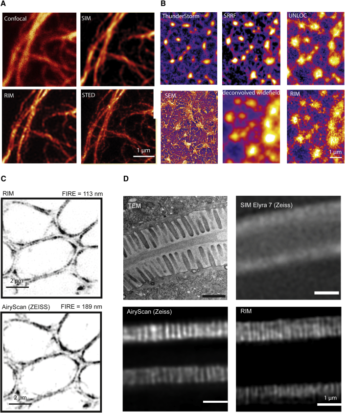
Comparison of RIM with competing super-resolution microscopy techniques (A) We imaged the same vimentin network from fixed HUVEC cell with, successively, 2D SIM, RIM, confocal, and 2D-STED, using a fl...
Figureu00a03
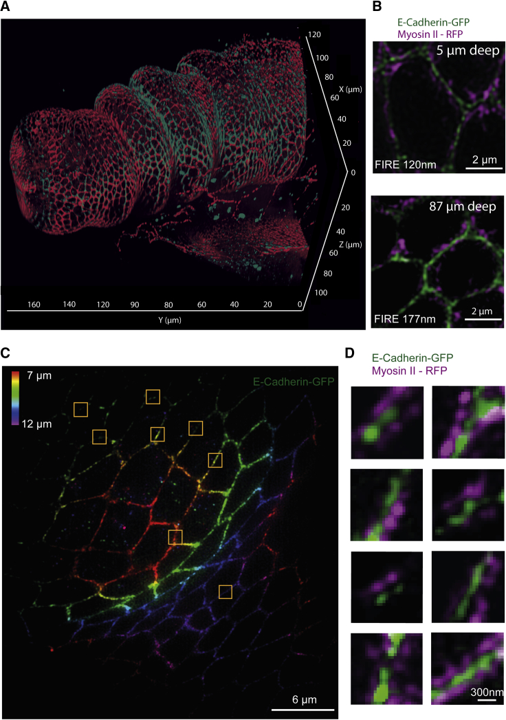
3D two-color imaging of a fixed Drosophila melanogaster leg (A) RIM 3D two-color imaging of a whole fixed Drosophila melanogaster pupa leg (see the cartoon in Figureu00a01 F) with (red or magenta) RFP...
Figureu00a04
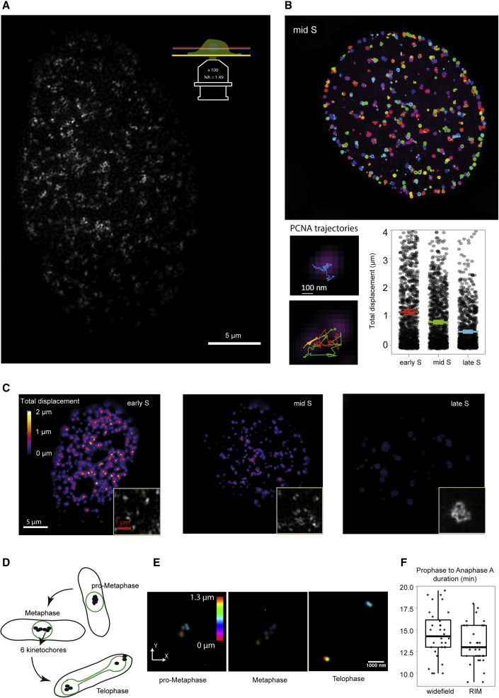
Dynamic imaging of cell nuclei (A) RIM image at 4u00a0u03bcm from the slide of the whole nucleus of a U2OS cell expressing mCherry-PCNA at early S phase. (B) Top: trajectories of individual spots of P...
Figureu00a05
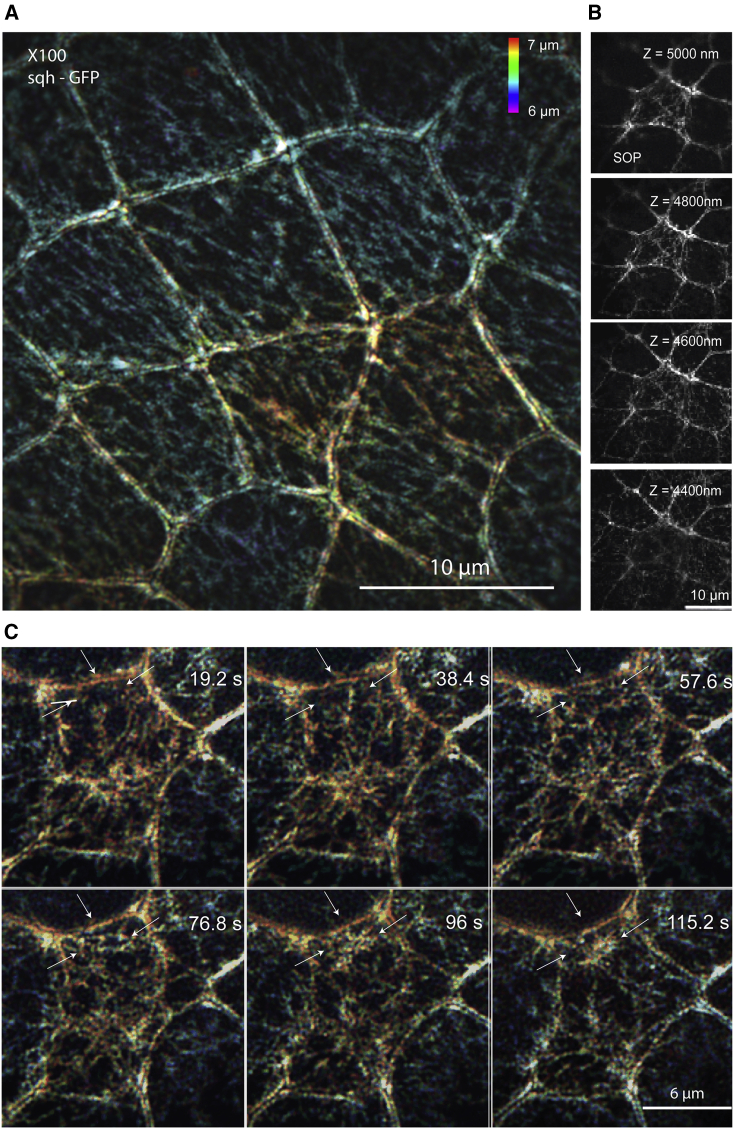
dynamic imaging of myosin II in live Drosophila notum (A) RIM 3D large field of view of the medial and junctional myosin II network at the apical plane of the columnar epithelium (extracted from Video...
Figure images are served from the NIH/NLM PubMed Central Open Access Subset or Europe PMC; copyright remains with the publishers and authors.
💬 Discussion
0 commentsNo comments yet. Be the first to start a discussion!
Leave a Comment